CHAPTER
3
Graphical Solution Method and Basic Optimization
Concepts
Solve the following problems using the graphical method. (3.1–3.10)
3.1_________________________________________________________________________________
Minimize (1,2)=(1−3)2+(2−3)2
Subject to 1+2≤4
1,2≥0
Solution
( ) ( )
22
12
112
21
32
3 3 ;
g 4 0;
g 0;
g0
fx x
xx
x
x
=−+−
= + −≤
=−≤
=−≤
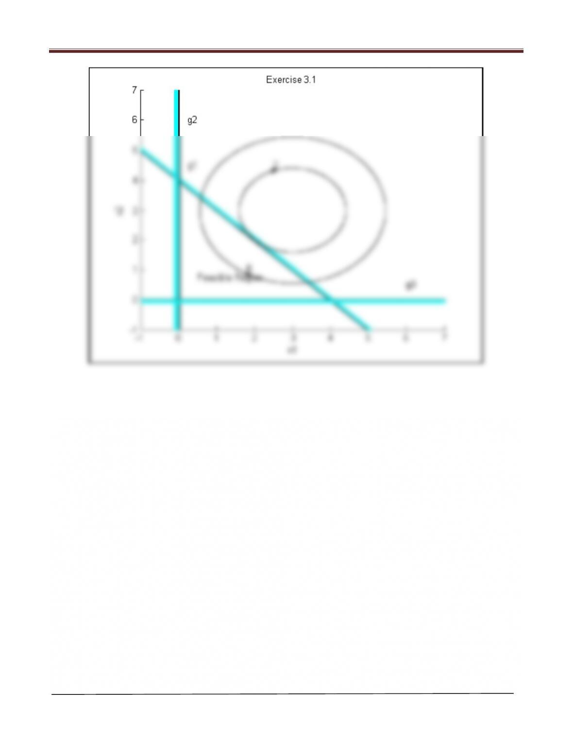
The optimum solution is:
12
2.0, 2.0, 2.0xxf
∗∗ ∗
= = =
Active constraint: g1
Chapter 3 Graphical Optimization and Basic Concepts
Arora, Introduction to Optimum Design, 4e
3-2
Chapter 3 Graphical Optimization and Basic Concepts
MATLAB Code
%Create a grid from -1 to 7 with an increment of 0.01 for the variables x1 and x2
[x1,x2]=meshgrid(-1:0.01:7.0, -1:0.01:7.0);
%Enter functions for the minimization problem
f=(x1-3).^2+(x2-3).^2;
xlabel(‘x1’),ylabel(‘x2’) %Specifies labels for x– and y-axes
hold on %retains the current plot and axes properties for all subsequent plots
%Use the “contour” command to plot constraint/minimization functions
cv1=[0 0]; %Specifies two contour values
const1=contour(x1,x2,g1,cv1,’k’,’LineWidth’,3); %Plots two specified contours of g1; k=black color
text(0.25,4.5,’g1′) %Writes g1 at the location (0.25, 4.5)
cv11=[0.01:0.01:0.1];
const1=contour(x1,x2,g1,cv11,’c’);
text(0.5,0.75,’Feasible Region’)
fv=[2 6]; %Defines contours for the minimization function
Arora, Introduction to Optimum Design, 4e
3-4
3.2________________________________________________________________________________
Maximize (1,2)=1+ 22
Subject to 21+2≤4
1,2≥0
Solution
=1+ 22;
3=−2≤0
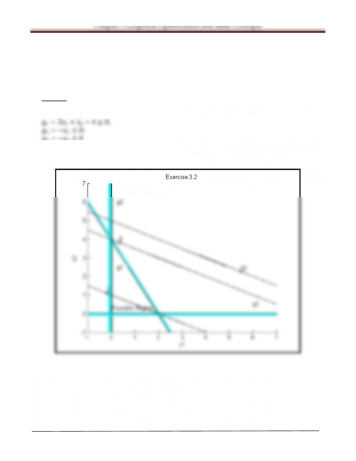
The optimum solution is:
12
0, 4, 8xxF
∗∗ ∗
= = =
. Active constraints: g1 and g2.
Chapter 3 Graphical Optimization and Basic Concepts
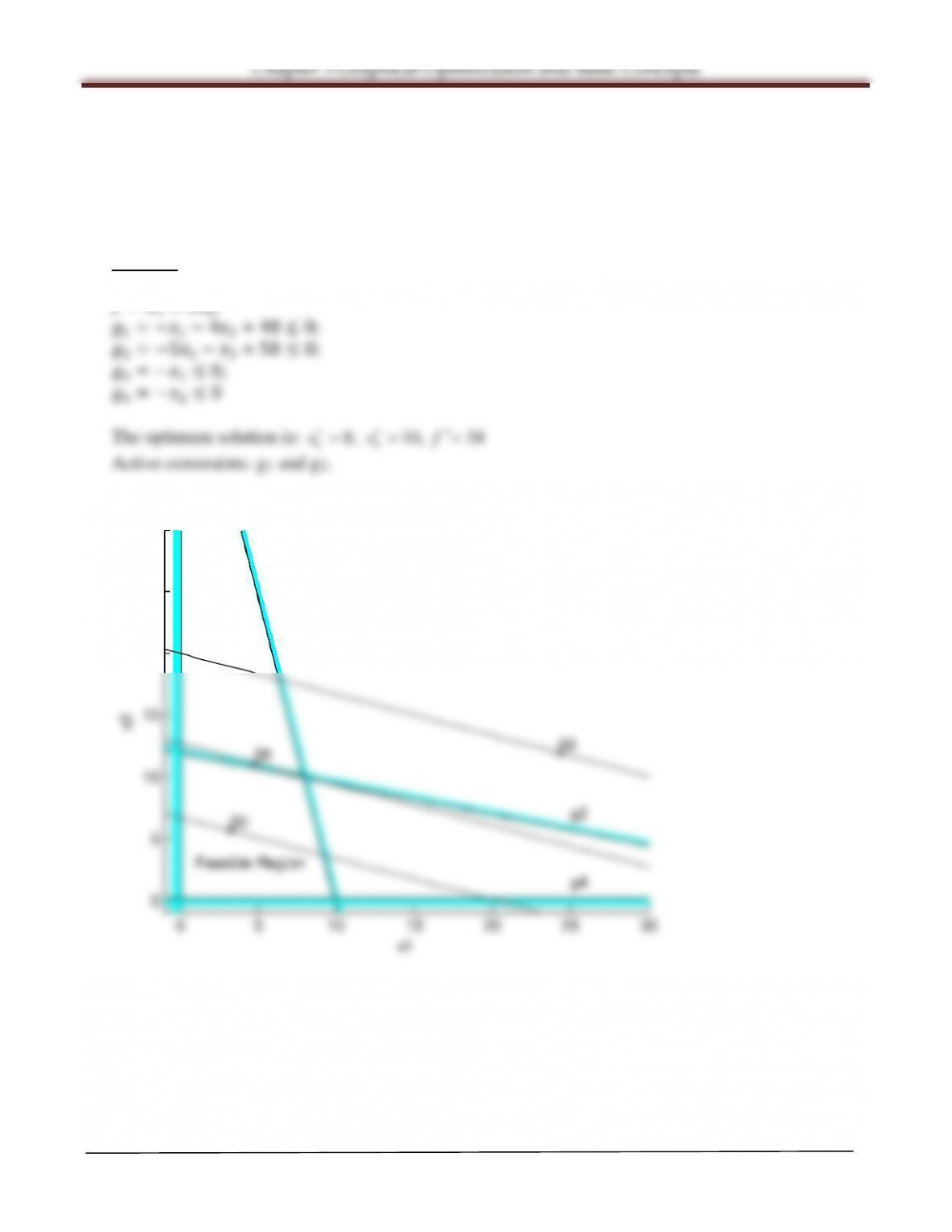
MATLAB Code for Exercise 3.2
%Create a grid from -1 to 7 with an increment of 0.01 for the variables x1 and x2
[x1,x2]=meshgrid(-1:0.01:7.0, -1:0.01:7.0);
%Enter functions for the minimization problem
text(0.25,2.5,’g1′)
cv11=[0.01:0.01:0.1];
const1=contour(x1,x2,g1,cv11,’c’);
text(0.05,0.3,’Feasible Region’)
fv=[2 8 10]; %Defines contours for the minimization function
Arora, Introduction to Optimum Design, 4e
3-6
3.3_________________________________________________________________________________
Minimize (1,2)=1+ 32
Subject to 1+ 42≥48
51+2≥50
1,2≥0
Solution
=1+ 32;
0 5 10 15 20 25 30
0
5
10
15
20
25
30
x1
x2
Exercise 3.3g1
g2
g4
g3
Feasible Region
20
38 60
Chapter 3 Graphical Optimization and Basic Concepts
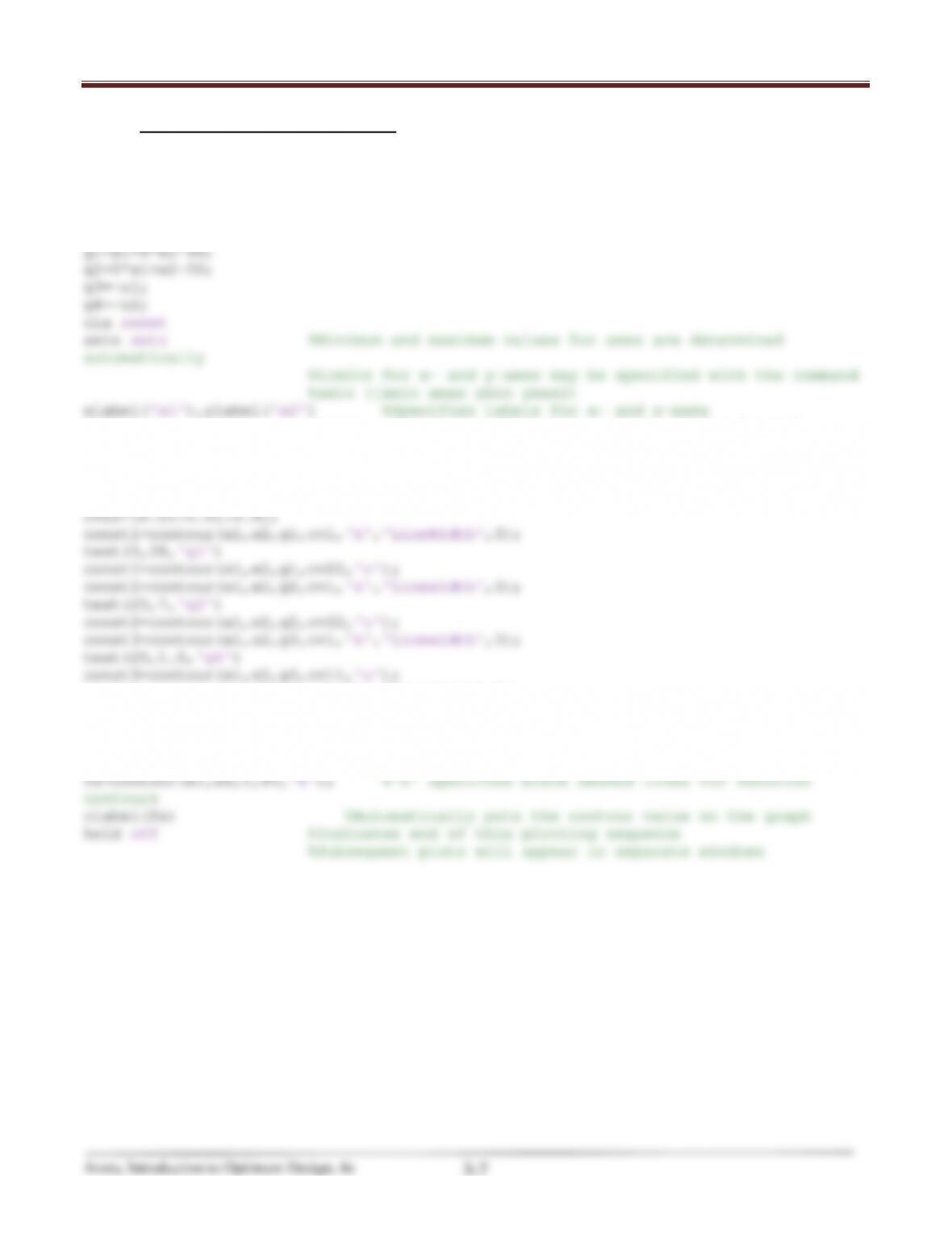
MATLAB Code for Exercise 3.3
%Exercise 3.3
%Create a grid from –1 to 30 with an increment of 0.5 for the variables x1 and x2
[x1,x2]=meshgrid(–1:0.5:30.0, –1:0.5:30.0);
%Enter functions for the minimization problem
f=x1+3*x2;
hold on %retains the current plot and axes properties for all
subsequent plots
text(15,28,‘Exercise 3.3’)
cv1=[0 0];
cv11=[0.01:0.01:0.4];
const4=contour(x1,x2,g4,cv1,‘k’,‘LineWidth’,3);
text(.75,29,‘g3’)
const4=contour(x1,x2,g4,cv11,‘c’);
text(1,3,‘Feasible Region’)
fv=[20 38 60]; %Defines contours for the minimization function
Chapter 3 Graphical Optimization and Basic Concepts
3.4 _________________________________________________________________________________
Maximize (1,2)=1+2+ 23
Subject to 1≤ 1≤4
32−23= 6
−1≤ 3≤2
2≥0
Solution
2 22
Rewrite the problem in the standard form with the remaining 2 design variables:
12
11
21
32
42
4 6;
g 1 0;
g 4 0;
g 4 3 0;
g 10 3 0
fxx
x
x
x
x
=−− +
=− +≤
= −≤
=−+ ≤
=−≤
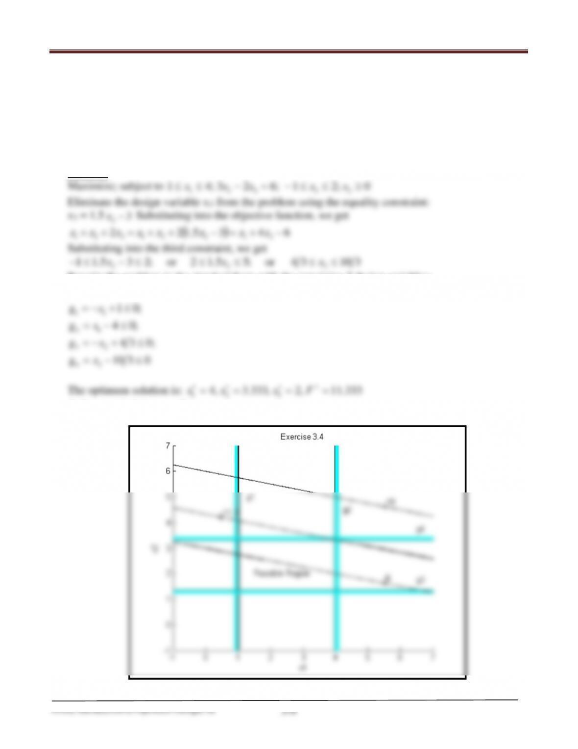
The optimum solution is:
12 3
4, 3.333, 2, 11.333xx xF
∗∗ ∗ ∗
= = = =
Active constraints: g2 and g4.
MATLAB Code for Exercise 3.4
%Create a grid from -1 to 7 with an increment of 0.01 for the variables x1 and x2
[x1,x2]=meshgrid(-1:0.01:7.0, -1:0.01:7.0);
%Enter functions for the minimization problem
text(1.25,5,’g1′)
cv11=[0.01:0.01:0.1];
text(6.5,3.75,’g4′)
text(4.25,4.5,’g2′)
text(6.5,1.75,’g3′)
text(1.5,2,’Feasible Region’)
fv=[-6 -11.333 -18]; %Defines contours for the minimization function
3.5 _________________________________________________________________________________
Maximize F(1,2)= 412
Subject to 1+2≤20
2− 1≤10
1,2≥0
Solution
12
112
2 21
31
42
4 ;
g 20 0;
g 10 0;
g 0;
g0
F xx
xx
xx
x
x
=
=+− ≤
= −− ≤
=−≤
=−≤
12
∗∗ ∗
Active constraint: g1.
0 5 10 15 20 25
0
5
10
15
20
25
x1
x2
Exercise 3.5
g1
g2
g4
g3
Feasible Region
100
250
400
700
Chapter 3 Graphical Optimization and Basic Concepts
MATLAB Code for Exercise 3.5
%Exercise 3.5
%Create a grid from –1 to 7 with an increment of 0.01 for the variables x1 and x2
[x1,x2]=meshgrid(–1:0.5:25.0, –1:0.5:25.0);
%Enter functions for the minimization problem
text(1.35,20,‘g1’)
cv11=[0.01:0.01:0.3];
cv22=[0.01:0.01:0.3];
text(0.3,23,‘g3’)
const4=contour(x1,x2,g4,cv22,‘c’);
text(1.5,2,‘Feasible Region’)
fv=[100 250 400 700]; %Defines contours for the minimization function
3.6 _________________________________________________________________________________
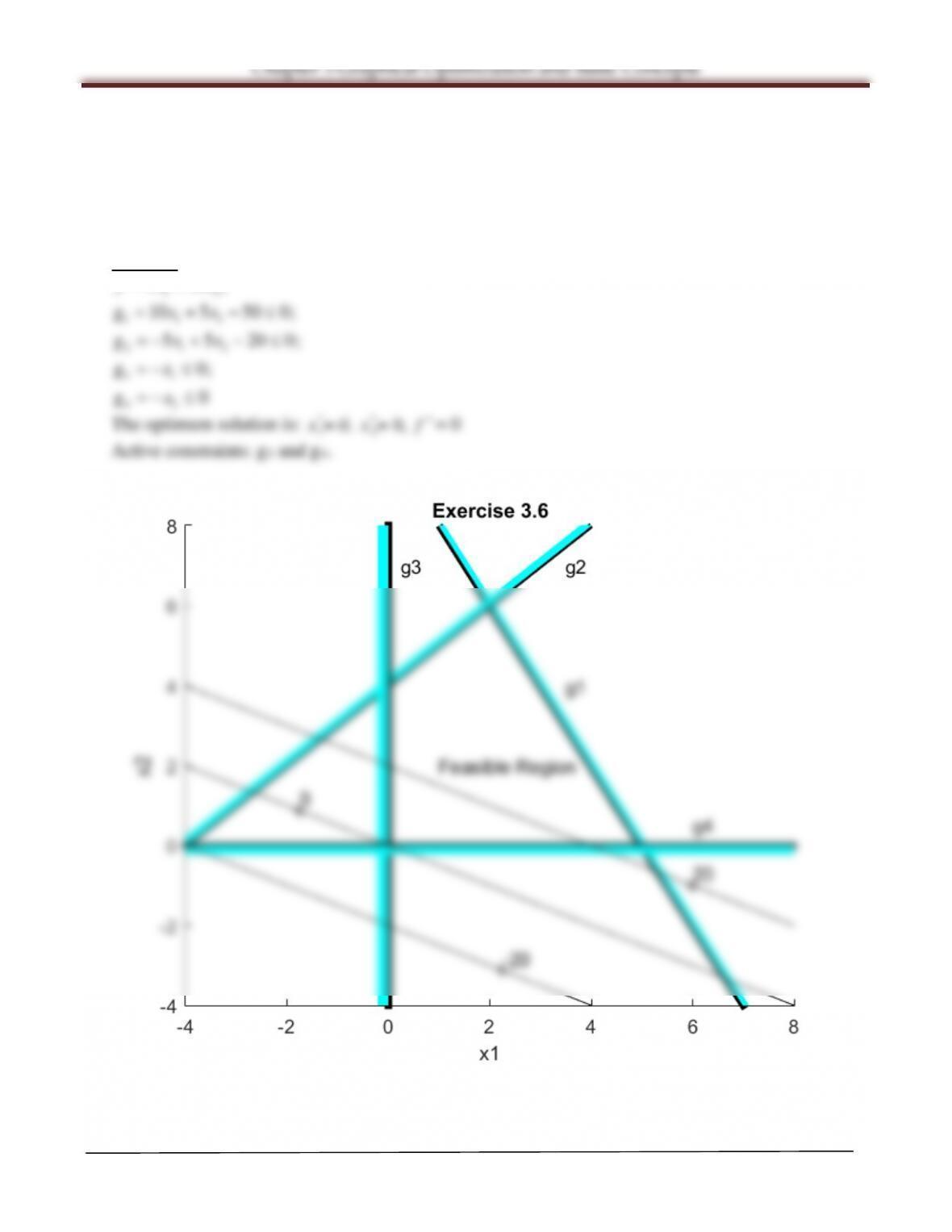
Minimize (1,2)= 51+102
Subject to 101+ 52≤50
51−52≥ −20
1,2≥0
Solution
12
1 12
2 12
31
42
5 10 ;
g 10 5 50 0;
g 5 5 20 0;
g 0;
g0
fx x
xx
xx
x
x
= +
= + −≤
=−+ −≤
=−≤
=−≤
The optimum solution is:
**
12
0, x = 0 , x = f ∗
= 0
Active constraints: g3 and g4.
Chapter 3 Graphical Optimization and Basic Concepts
MATLAB Code
%Exercise 3.6
%Create a grid from -1 to 7 with an increment of 0.01 for the variables x1 and x2
[x1,x2]=meshgrid(-4:0.5:8.0, -4:0.5:8.0);
%Enter functions for the minimization problem
f=5*x1+10*x2;
text(3.5,4,’g1′)
text(3.5,7,’g2′)
text(0.25,6,’g3‘)
const4=contour(x1,x2,g4,cv1,’k’,’LineWidth’,3);
text(7,0.25,’g4‘)
Chapter 3 Graphical Optimization and Basic Concepts
3.7 _________________________________________________________________________________
Minimize (1,2)= 31+2
Subject to 21+ 42≤21
51+ 32≤18
1,2≥0
Solution
12
112
2 12
31
42
3 ;
g 2 4 21 0;
g 5 3 18 0;
g 0;
g0
f xx
xx
xx
x
x
= +
= + −≤
= + −≤
=−≤
=−≤
The optimum solution is: x
12
0, 0, 0x f
∗∗ ∗
= = =
Active constraints: g3 and g4.
-2 02468
-2
-1
0
1
2
3
4
5
6
7
8
x1
x2
Exercise 3.7
g1
g2
g4
g3
Feasible Region
-5
0
5
Chapter 3 Graphical Optimization and Basic Concepts
MATLAB Code
%Exercise 3.7
%Create a grid from –1 to 7 with an increment of 0.01 for the variables x1 and x2
[x1,x2]=meshgrid(–2:0.5:8.0, –2:0.5:8.0);
%Enter functions for the minimization problem
f=3*x1+x2;
text(3.5,4.1,‘g1’)
text(2.5,2.5,‘g2’)
cv34=[0.01:0.01:0.2];
text(0.25,0.75,‘Feasible Region’)
fv=[–5 0 5]; %Defines contours for the minimization function
Chapter 3 Graphical Optimization and Basic Concepts
3.8 _________________________________________________________________________________
Minimize (1,2)=1
2−22
2−41
Subject to 1+2≤6
2≤3
1,2≥0
Solution
22
1 21
112
22
31
42
2 4 (hyperbola);
g 6 0;
g 3 0;
g 0;
g0
fxxx
xx
x
x
x
=−−
= + −≤
= −≤
=−≤
=−≤
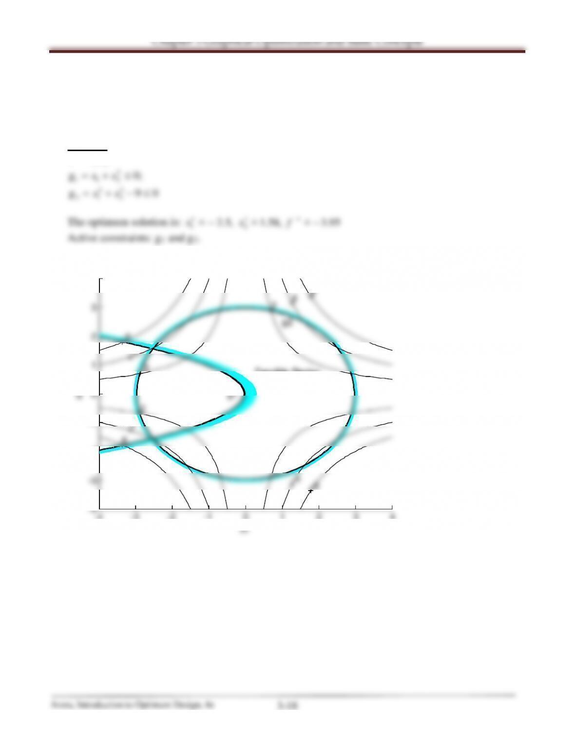
The optimum solution is:
12
2, 3, 22xx f
∗∗ ∗
= = = −
Active constraint: g1.
-2
-1
0
1
2
3
4
5
6
7
8
x2
Exercise 3.8
g1
g2
g4
g3
Feasible Region
–35
–22
–15
-4
-4
Chapter 3 Graphical Optimization and Basic Concepts
MATLAB Code
%Exercise 3.8
%Create a grid from –1 to 7 with an increment of 0.01 for the variables x1 and x2
hold on
cv1=[0 0];
cv12=[0.01:0.01:0.3];
const1=contour(x1,x2,g1,cv1,‘k’,‘LineWidth’,4);
text(2.5,4.5,‘g1’)
text(1.2,2.7,‘g2’)
cv34=[0.01:0.01:0.2];
text(0.25,7,‘g3’)
const4=contour(x1,x2,g4,cv34,‘c’);
text(0.5,1.25,‘Feasible Region’)
fv=[–4 –15 –22 –35]; %Defines contours for the minimization function
3.9 _________________________________________________________________________________
Minimize (1,2)=12
Subject to 1+2
2≤0
1
2+2
2≤9
Solution
12
2
112
22
21 2
;
g 0;
g 90
f xx
xx
xx
=
=+≤
= + −≤
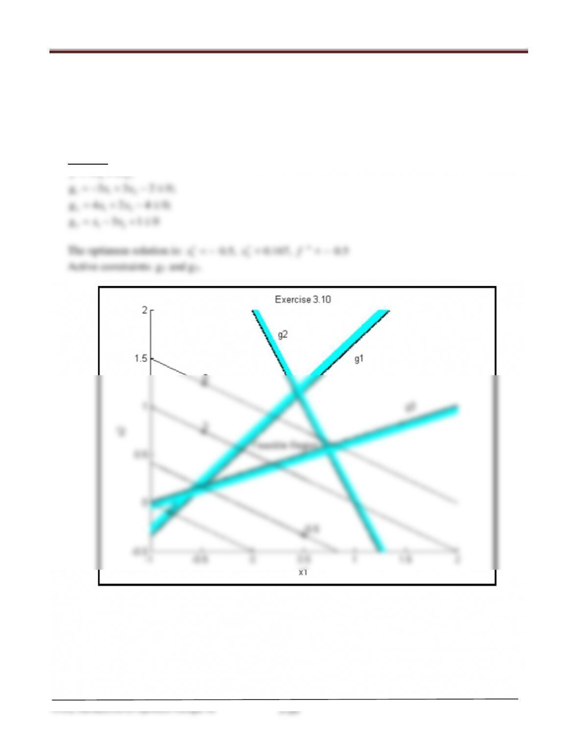
The optimum solution is:
12
2.5, 1.58, 3.95x xf
∗∗∗
=−= =−
Active constraints: g1 and g2.
-4 -3 -2 -1 01234
-4
-3
-2
-1
0
1
2
3
4
x1
x2
Exercise 3.9
g1
g2
Feasible Region
-6
-6
-4
-4
-2
-2
2
2
4
4
6
6
Chapter 3 Graphical Optimization and Basic Concepts
MATLAB Code
%Exercise 3.9
f=x1.*x2;
g1=x1+x2.^2;
g2=x1.^2+x2.^2–9;
cla reset
text(0.25,0.75,‘Feasible Region’)
fv=[2 –2 4 –4 6 –6]; %Defines contours for the minimization function
Chapter 3 Graphical Optimization and Basic Concepts
3.10 ________________________________________________________________________________
Minimize (1,2)= 31+ 62
Subject to −31+ 32≤2
41+ 22≤4
−1+ 32≥1
Solution
12
1 12
2 12
31 2
= 3 + 6 ;
g 3 3 2 0;
g 4 2 4 0;
g 3 10
fxx
xx
xx
xx
=− + −≤
= + −≤
= − +≤
The optimum solution is:
12
0.5, 0.167, 0.5xxf
∗∗ ∗
=−= =−
Active constraints: g1 and g3.