Aeronautical Engineering Chapter 3 Arora Introduction Optimum Design Graphical Solution Method And Basic Optimization Concepts

Arora, Introduction to Optimum Design, 4e

3-101

3.41________________________________________________________________________________

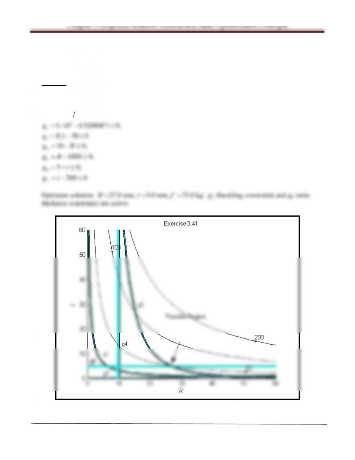
Solve Exercise 3.23 for a column fixed at one end and pinned at the other. The buckling load for a

column is given as 22/2. Use graphical method.

Solution

Referring to Exercise 3.23, this problem is formulated as follows: (only the buckling load constraint

is changed; buckling load is 8 times of that in Exercise 3.23):

f = 0.2466Rt;

1

43

2

3

g 7957.7 250 0;

g 5 10 0.52088 0;

g 50 0

Rt

= −≤

=×− ≤

= −≤

4

5

6

7

g 10 0;

g 1000 0;

g 5 0;

g 200 0

R

t

= −≤

=−≤

= −≤

=−≤

Optimum solution: R

=

∗

27.0 mm, t

=

∗

5.0 mm, f

=

∗

33.0 kg; g2 (buckling constraint) and g6 (min.

thickness constraint) are active.

Chapter 3 Graphical Solution Method and Basic Optimization Concepts

MATLAB Code

[R,t]=meshgrid(0:1:60, 0:1:60);

%Enter functions for the minimization problem

f=0.2466*R.*t;

g1=7957.7-250*R.*t;

g2=5*10^4-0.52088*(R.^3).*t;

g3=R-50*t;

g4=10-R;

cv11=[0.01:0.01:0.5];

const1=contour(R,t,g1,cv11,’c’);

const2=contour(R,t,g2,cv1,’k’,’Linewidth’,3);

const2=contour(R,t,g2,cv11,’c’);

text(16,30,’g2′)

text(0.9,7,’g6′)

const7=contour(R,t,g7,cv1,’k’,’Linewidth’,3);

const7=contour(R,t,g7,cv11,’c’);

Arora, Introduction to Optimum Design, 4e

3-103

3.42________________________________________________________________________________

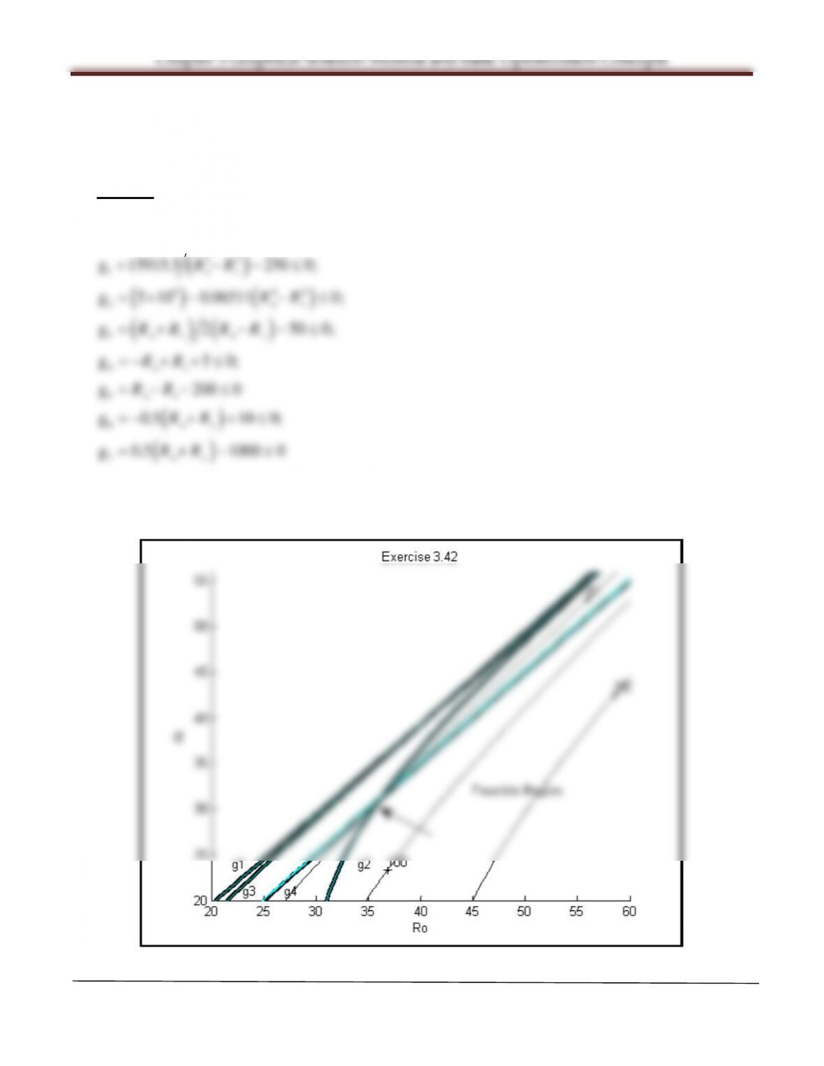
Solve Exercise 3.24 for a column pinned at both ends. The buckling load for such a column is given

as 2/2. Use the graphical method.

Solution

Referring to Exercise 3.24, the problem is formulated as follows:

f = 0.1233

( )

22

oi

RR−

;

( )

( ) ( )

22

1 oi

5 44

2 oi

g 15915.5 250 0;

g 5 10 0.06511 0;

RR

= −−≤

=×− −≤

( ) ( )

3 oi oi

4 oi

5 oi

g 2 50 0;

g 5 0;

g 200 0

RR RR

RR

= + − −≤

=− + +≤

=−− ≤

( )

6 oi

7 oi

g 0.5 10 0;

g 0.5 1000 0

RR

=− + +≤

= +− ≤

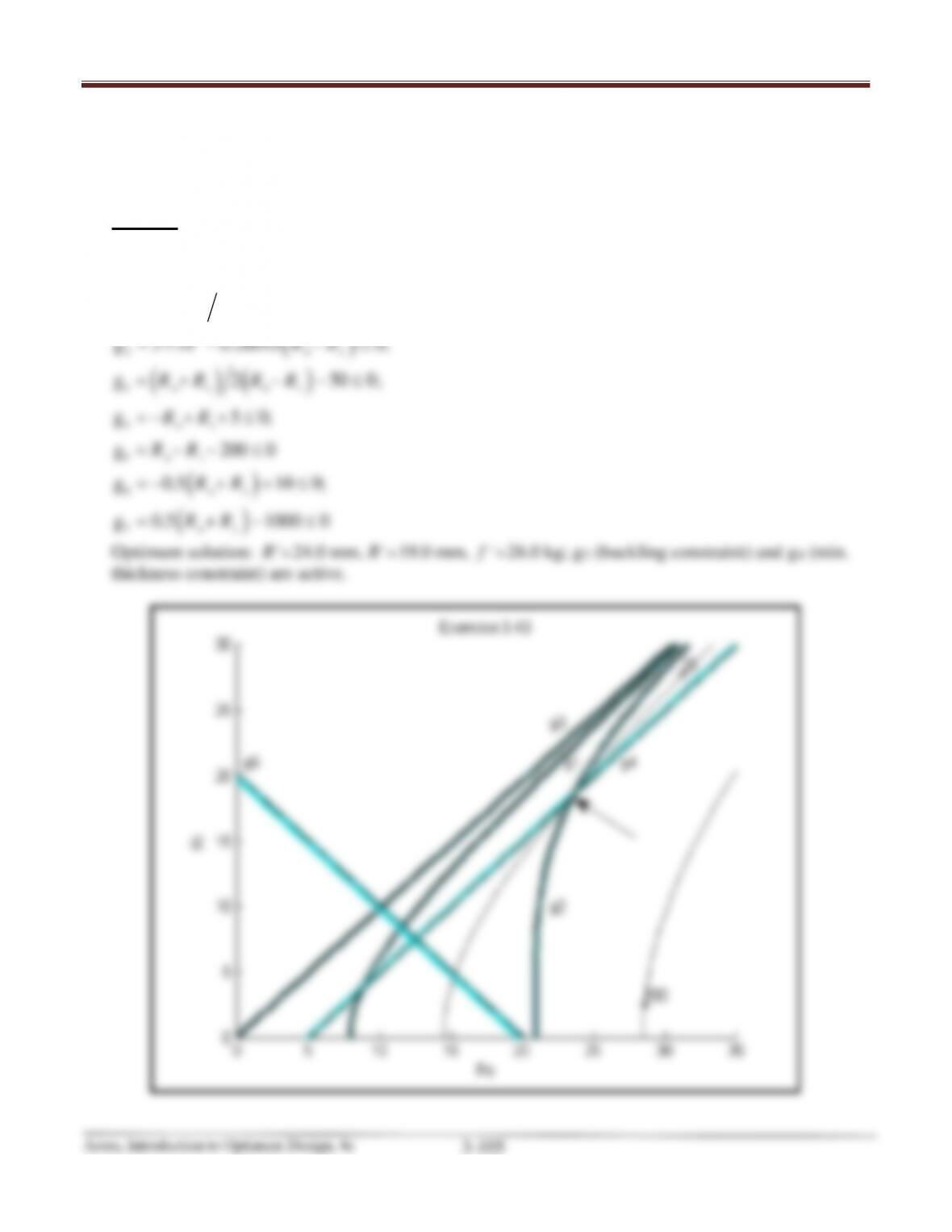
Optimum solution: R

=

∗

o

36 mm, R

=

∗

i

31 mm, f

∗=



41 kg; g2 (buckling constraint) and g4 (minimum

thickness) are active.

Chapter 3 Graphical Solution Method and Basic Optimization Concepts

MATLAB Code

[Ro,Ri]=meshgrid(20:1:60, 20:1:56);

%Enter functions for the minimization problem

f=0.1233*(Ro.^2-Ri.^2);

g1=15915.5-250*(Ro.^2-Ri.^2);

g2=5*10^4-0.06511*(Ro.^4-Ri.^4);

g3=(Ro+Ri)-100*(Ro-Ri);

g4=5–Ro+Ri;

cv11=[0.01:0.01:0.2];

const1=contour(Ro,Ri,g1,cv11,’c’);

const2=contour(Ro,Ri,g2,cv1,’k’,’Linewidth’,3);

const2=contour(Ro,Ri,g2,cv11,’c’);

text(34,24,’g2′)

const6=contour(Ro,Ri,g6,cv11,’c’);

text(0,7,’g6′)

const7=contour(Ro,Ri,g7,cv1,’k’,’Linewidth’,3);

const7=contour(Ro,Ri,g7,cv11,’c’);

text(6,200,’g7′)

Chapter 3 Graphical Solution Method and Basic Optimization Concepts

3.43________________________________________________________________________________

Solve Exercise 3.24 for a column pinned at both ends. The buckling load for such a column is given

as 42/2. Use the graphical method.

Solution

Referring to Exercise 3.24, this problem is formulated as follows:

f = 0.1233

( )

22

oi

RR−

( )

22

1 oi

4 44

2 oi

g 15915.5 250 0;

g 5 10 0.26045 0;

RR

= −−≤

=×− − ≤

( ) ( )

3 oi oi

4 oi

5 oi

g 2 50 0;

g 5 0;

g 200 0

RR RR

RR

= + − −≤

=− + +≤

=−− ≤

( )

6 oi

7 oi

g 0.5 10 0;

g 0.5 1000 0

RR

=− + +≤

= +− ≤

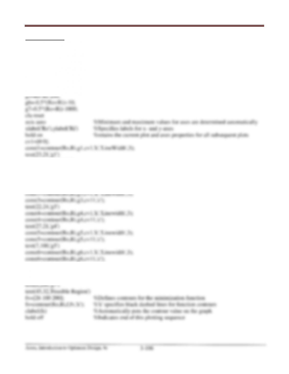
Optimum solution: R

=

∗

24.0 mm, R

=

∗



19.0 mm, f

=

∗



26.0 kg; g2 (buckling constraint) and g4 (min.

thickness constraint) are active.

Chapter 3 Graphical Solution Method and Basic Optimization Concepts

MATLAB Code

[Ro,Ri]=meshgrid(0:1:35, 0:1:30);

%Enter functions for the minimization problem

f=0.1233*(Ro.^2-Ri.^2);

g1=15915.5-250*(Ro.^2-Ri.^2);

g2=5*10^4-0.26045*(Ro.^4-Ri.^4);

g3=(Ro+Ri)-100*(Ro-Ri);

g4=5-Ro+Ri;

cv11=[0.01:0.01:0.2];

const1=contour(Ro,Ri,g1,cv11,’c’);

const2=contour(Ro,Ri,g2,cv1,’k’,’Linewidth’,3);

const2=contour(Ro,Ri,g2,cv11,’c’);

text(22,10,’g2′)

text(0.5,21,’g6′)

const7=contour(Ro,Ri,g7,cv1,’k’,’Linewidth’,3);

const7=contour(Ro,Ri,g7,cv11,’c’);

3.44________________________________________________________________________________

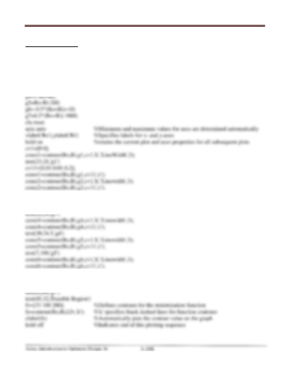
Solve Exercise 3.24 for a column fixed at one end and pinned at the other. The buckling load for

such a column is given as 22/2. Use the graphical method.

Solution

Chapter 3 Graphical Solution Method and Basic Optimization Concepts

MATLAB Code: 3.44

[Ro,Ri]=meshgrid(0:1:35, 0:1:27);

%Enter functions for the minimization problem

f=0.1233*(Ro.^2-Ri.^2);

g1=15915.5-250*(Ro.^2-Ri.^2);

g2=5*10^4-0.13022*(Ro.^4-Ri.^4);

g3=(Ro+Ri)-100*(Ro-Ri);

text(25.5,10,’g2′)

const3=contour(Ro,Ri,g3,cv1,’k’,’Linewidth’,3);

const3=contour(Ro,Ri,g3,cv11,’c’);

text(0.5,21,’g6′)

const7=contour(Ro,Ri,g7,cv1,’k’,’Linewidth’,3);

const7=contour(Ro,Ri,g7,cv11,’c’);

Chapter 3 Graphical Solution Method and Basic Optimization Concepts

Arora, Introduction to Optimum Design, 4e

3-109

3.45________________________________________________________________________________

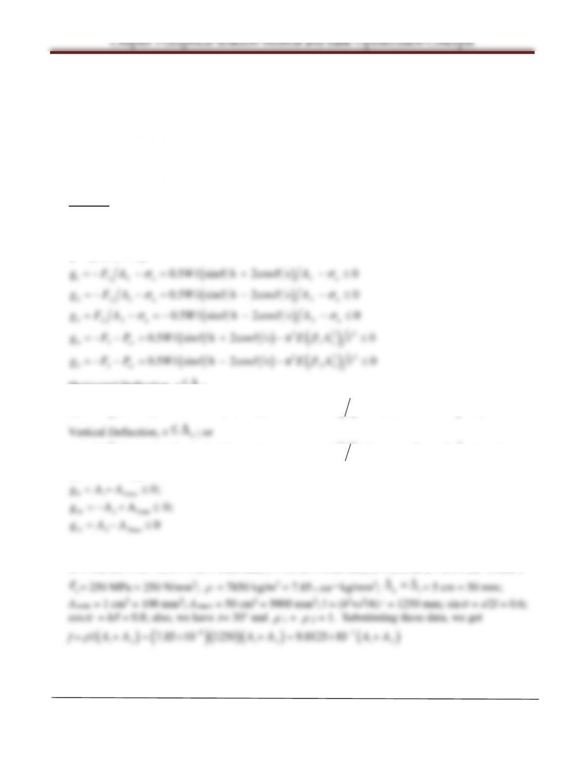
Solve the can design problem formulated in Section 2.2 using the graphical approach.

Solution

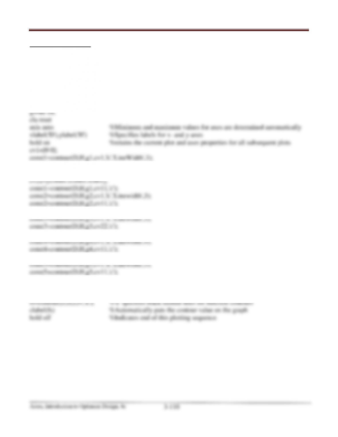
Referring to Section 2.2, the problem is formulated as follows:

Constraints:

2

1

2

3

4

g 400 π 4 0;

g 3.5 0;

g 8.0 0;

DH

D

H

=−≤

= −≤

=−≤

= −≤

5

g 18.0 0H=−≤

∗

Chapter 3 Graphical Solution Method and Basic Optimization Concepts

MATLAB Code: 3.45

[D,H]=meshgrid(7.97:0.001:8.02, 7.7:0.001:8.2);

%Enter functions for the minimization problem

f=pi*D.*H+0.5*pi*(D.^2);

g1=400-0.25*pi*(D.^2).*H;

g2=3.5-D;

g3=D-8;

g4=8–H;

text(8.015,7.95,’g1′)

cv11=[0.001:0.001:0.01];

text(0.85,1000,’g2′)

text(7.997,8.15,’g3′)

text(8.01,8.02,’g4′)

text(2.2,21,’g5′)

text(7.985,8.15,’Feasible Region’)

fv=[300 301.6 303]; %Defines contours for the minimization function

3.46________________________________________________________________________________

Consider the two–bar truss shown in Figure 2.5. Using the given data, design a minimum mass

structure where W = 100 kN;  = 30°; h = 1 m; s = 1.5 m; modulus of elasticity, E = 210 GPa;

allowable stress,  = 250 MPa, mass density,  = 7850 kg/m3. Use Newtons and millimeters as

units. The members should not fail on stress and their buckling should be avoided. Deflection at the

top in either direction should not be more than 5 cm.

Use cross –sectional area A1 and A2 of the two members as design variables and let the moment

of inertia of the members be given as I = A2. Area must also satisfy the constraint 1≤Ai≤50cm2.

Solution

Consider the two bar truss shown in Figure 2.5 and refer to the formulation in Section 2.5. Using the

cross–sectional areas A1 and A2 of the two members as design variables, this problem can be

formulated as follows:

( )

1 2

1 1 1 1

2 2 2 2

3 2 2 2

2 22

4 1 cr 1 1

2

5 2 cr

= ( )

g 0.5 sin 2cos 0

g 0.5 sin 2cos π0

g 0.5 sin 2cos π

aa

f lA A

F A Wl h s A

F P Wl h s E A l

F P Wl h s E

+

=− −= + −≤

=− −= − −≤

= −=− − −≤

=−− = + − ≤

=−− = − −

ρ

σ θθσ

θθ β

( )

22

0Al≤

Horizontal Deflection, u

Δu

≤

;

( ) ( )

2 22

6 1 2 1 2 12

g cos cos sin cos sin 4 sin cos Δ0

u

Wl A A A A EA A



= + −− −≤

αθ ααθ α α

( ) ( )

2 22

7 1 2 1 2 12

8 1 1min

9 1 1max

10 2 2min

11 2 2max

g sin sin sin cos cos 4 sin cos Δ0

g 0;

g A 0;

g0

v

Wl A A A A EA A

AA

A

AA

αθ ααθ α α



= + −− −≤



=−+ ≤

=−≤

=−+ ≤

=−≤

Use kilograms, Newtons and millimeters as units for the given data:

W = 100 kN = 105 N; h = 1 m = 1000 mm; s = 1.5 m = 1500 mm; E = 210 GPa = 2.1

5

10×

N/mm2;

a

σ

= 250 MPa = 250 N/mm2;

ρ

= 7850 kg/m3 = 7.85

6

10

−

×

kg/mm3;

ΔΔ

uv

=

= 5 cm = 50 mm;

Aimin = 1 cm2 = 100 mm2; Aimax = 50 cm2 = 5000 mm2; l = (h2+s2/4)

2

1

= 1250 mm; sin

α

= s/2l = 0.6;

cos

α

= h/l = 0.8; also, we have

θ

= 30° and

β

1 =

β

2 = 1. Substituting these data, we get

f =

( )

( )( ) ( )

63

12 12 12

7.85 10 1250 9.8125 10lAA AA AA

−−

+= × += × +

ρ

Chapter 3 Graphical Solution Method and Basic Optimization Concepts

11

22

32

g 103420 250 0;

g 40925 250 0;

A

= −≤

=− −≤

= −≤

52

41

g 1.034188 10 1.32647 0A= ×− ≤

Constraint g5 is neglected, since the corresponding bar is subjected to tensile force.

( ) ( )

6 1 2 12

g 202.97 512.95A A AA= +

;

( ) ( )

7 1 2 12

g 150.22275 383.474 50 0A A AA=− + −≤

81

91

10 2

11 2

g 100 0;

g 5000 0;

g 100 0;

g 5000 0

A

= −≤

=−≤

= −≤

=−≤

Neglecting the redundant constraints, i.e., g2, g4, g5, g7, g8 and g10, and rearranging the constraints

we get the formulation as follows:

3

11

22

g 103420 250 0;

g 40925 250 0

A

= −≤

Optimum solution: A

=

∗

1

413.68 mm, A

=

∗

2

163.7 mm, f

∗

= 5.7 kg; g1(stress constraint of member 1)

and g2(horizontal deflection constraint) are active.

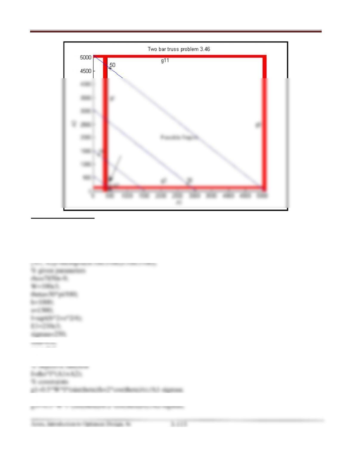
Chapter 3 Graphical Solution Method and Basic Optimization Concepts

MATLAB Code: 3.46

% Problem 3.46

% Hyeongjin Song

clear all;

% define mesh for A1 and A2

cosa=0.8;

delta=50;

g2=0.5*W*l*(sin(theta)/h-2*cos(theta)/s)./A2-sigmaa;

Chapter 3 Graphical Solution Method and Basic Optimization Concepts

Arora, Introduction to Optimum Design, 4e

3-115

hold off

Chapter 3 Graphical Solution Method and Basic Optimization Concepts

Arora, Introduction to Optimum Design, 4e

3-116

3.47________________________________________________________________________________

For Exercise 3.46, use the hollow circular tubes as members with mean radius R and wall thickness t

as design variables. Make sure that R/t ≤ 50. Design the structure so that member 1 is symmetric

with member 2. The radius and thickness must also satisfy the constraints 2≤t≤40 mm and 2≤R≤40

cm.

Solution

Consider the two bar truss shown in Fig. 2.2 and refer to the formulation in Section 2.5. Using the

hollow circular tubes as members with mean radius R and wall thickness t as design variables, the

problem is formulated as follows:

f =

( )

2 22 4Al Rt l lRt= =

ρ ρ π πρ

( )

11

2 32

2 1 cr

g 0.5 sin 2cos 2 π0

g 0.5 sin 2cos ππ 0

aa

F A W l h s Rt

F P Wl h s E R t l

=− −= + −≤

=−− = + − ≤

σ θθ σ

θθ

Horizontal Deflection, u

Δu

≤

;

( )

32

3

g cos π Δ0

u

Wl RtEs= −≤

θ

Vertical Deflection, v

Δv

≤

;

( )

32

4v

5

g sin 4π Δ 0;

g 50 0

W l RtEh

Rt

θ

= −≤

6 min

7 max

8 min

9 max

g 0;

g0

RR

tt

=−+ ≤

=−≤

=−+ ≤

=−≤

Substituting the data given in Exercise 3.46 and the following simple bounds, Rmin = 20 mm,

Rmax = 400 mm, tmin = 2 mm, tmax = 40 mm, we get

6

–

7

g 400 0;

R

=−≤

Chapter 3 Graphical Solution Method and Basic Optimization Concepts

8

9

g 2 0;

g 40 0

t

= −≤

=−≤

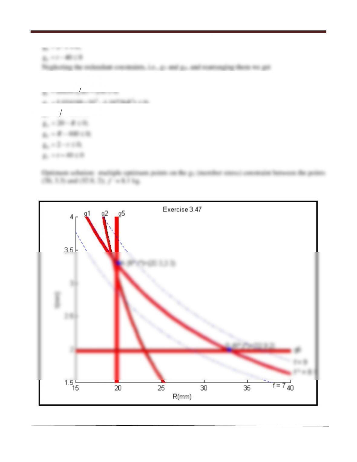
Neglecting the redundant constraints, i.e., g3 and g4, and rearranging them we get

f = 0.123308Rt ;

1

g 16459.5 250 0;

Rt

= −≤

Chapter 3 Graphical Solution Method and Basic Optimization Concepts

MATLAB Code: 3.47

f = 0.123308*R.*t;

g1 = (16459.5./(R.*t))-250;

g2 = 1.034188*10^5 – (4.16726*R.^3).*t;

g3 = R./t-50;

g4 = 20 – R;

text(16,4.05,’g1′)

cv11 = [0:0.1:5];

const1 = contour(R,t,g1,cv11,’r’);

cv2 = [0:100:300];

const2 = contour(R,t,g2,cv2,’k’);

text(20,4.05,’g5′)

cv44 = [0:0.01:0.4];

const4 = contour(R,t,g4,cv44,’r’);

%Not Shown in Figure

cv5 = [0 0];

text(40.5,2,’g6′)

Chapter 3 Graphical Solution Method and Basic Optimization Concepts

const6 = contour(R,t,g6,cv66,’r’);

text(20.2,3.3,’A (R*,t*)=(20.3,3.3)’);

text(32.5,2.05,’B (R*,t*)=(32.9,2)’);

fv=[7,8.1,9];

Chapter 3 Graphical Solution Method and Basic Optimization Concepts

3.48 ________________________________________________________________________________

Design a symmetric structure defined in Exercise 3.46 treating cross–sectional area A and height h as

design variables. The design variables must also satisfy the constraints 1 ≤A ≤50 cm2 and 0.5 ≤ h

≤3 m.

Solution

Refer to Fig. 2.1 and the formulation in Section 2.5. Treating cross-sectional area A (for each

member) and h as design variables, the problem is formulated as follows:

0.5

2

