Chapter 2 Optimum Design Problem Formulation
Arora, Introduction to Optimum Design, 4e
2-21
FORMULATION 1: In terms of intermediate variables
Step 3: Definition of Design Variables
H = height of the truss, m
0.1
2 m; 0.1 0.1 mDt≤ ≤ ≤≤
Chapter 2 Optimum Design Problem Formulation
FORMULATION 2: Explicitly in terms of the design variables.
Use N and m as the units, and the corresponding values for various parameters.
22
1
Step 3: Definition of Design Variables
H = height of the truss, m
Step 4: Optimization Criterion
Optimization criterion is to minimize mass, and the cost function is defined as
1
2
22
Substituting the given values, we get
1
2
2
2
2
1
2
2
1
Arora, Introduction to Optimum Design, 4e
2-23
2.17________________________________________________________________________________
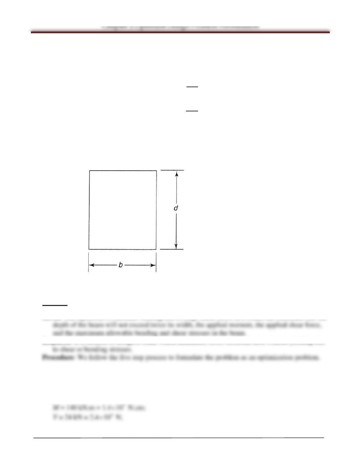
A beam of rectangular cross section (Fig. E2.17) is subjected to a maximum bending moment of M
and maximum shear of V. The allowable bending and shearing stresses are σa and τa, respectively.
The bending stress in the beam is calculated as
=6
2
and average shear stress in the beam is calculated as
τ=3
2
where d is the depth and b is the width of the beam. It is also desired that the depth of the beam shall
not exceed twice its width. Formulate the design problem for minimum cross–sectional area using
this data: M=140 kN
⋅
m, V=24 kN, =165 MPa, =50 MPa.
FIGURE E2.17 Cross section of a rectangular beam.
Solution
Given: The equations to calculate bending and average shear stress in a beam, the constraint that the
Required: It is desired to design a beam which minimizes cross-sectional area without yielding due
Step 1: Problem Statement
Shown above
Step 2: Data and Information Collection
7
Chapter 2 Optimum Design Problem Formulation
Arora, Introduction to Optimum Design, 4e
2-24
a
Step 3: Definition of Design Variables
Arora, Introduction to Optimum Design, 4e
2-25
2.18________________________________________________________________________________
A vegetable oil processor wishes to determine how much shortening, salad oil, and margarine to
produce to optimize the use of his current oil stock supply. At the present time, he has 250,000 kg of
soybean oil, 110,000 kg of cottonseed oil, and 2000 kg of milk–base substances. The milk–base
substances are required only in the production of margarine. There are certain processing losses
associated with each product: 10 percent for shortening, 5 percent for salad oil, and no loss for
margarine. The producer’s back orders require him to produce at least 100,000 kg of shortening,
50,000 kg of salad oil, and 10,000 kg of margarine. In addition, sales forecasts indicate a strong
demand for all produces in the near future. The profit per kilogram and the base stock required per
kilogram of each product are given in Table E2.18. Formulate the problem to maximize profit over
the next production scheduling period. (created by J. Liittschwager).
Table E2.18 Data for the Vegetable Oil Processing Problem
Parts per kg of base stock
Requirements
Product
Profit per kg
Soybean
Cottonseed
Milk base
Shortening
1.0
2
1
0
Salad oil
0.8
0
1
0
Margarine
0.5
3
1
1
Solution
Given: The current supply of soybean oil, cottonseed oil, and milk-base substances, milk–base
Step 1: Problem Statement
Shown above
Step 2: Data and Information Collection
Shown above
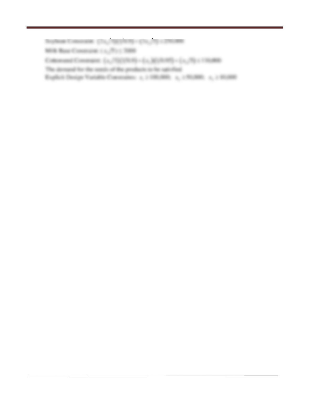
Step 3: Definition of Design Variables
Chapter 2 Optimum Design Problem Formulation
Arora, Introduction to Optimum Design, 4e
2-26
Chapter 2 Optimum Design Problem Formulation
Section 2.11 A General Mathematical Model for Optimum Design
2.19________________________________________________________________________________
Answer True or False.
2. All design problems have only linear inequality constraints. False
4. If there is an equality constraint in the design problem, the optimum solution must satisfy it. True
6. A feasible design may violate equality constraints. False
8. A “≤ type” constraint expressed in the standard form is active at a design point if it has zero
value there. True
10. The number of independent equality constraints can be larger than the number of design
variables for the problem. True
12. The feasible region for an equality constraint is a subset of that for the same constraint expressed
as an inequality. True
14. A lower minimum value for the cost function is obtained if more constraints are added to the
problem formulation. False
15. Let
be the minimum value for the cost function with n design variables for a problem. If the
Arora, Introduction to Optimum Design, 4e
2-28
2.20*_______________________________________________________________________________
A trucking company wants to purchase several new trucks. It has $2 million to spend. The
investment should yield a maximum of trucking capacity for each day in tonnes
×
kilometers. Data
for the three available truck models are given in Table E2.20: i.e., truck load capacity speed, crew
required/shift, hours of operations for three shifts, and the cost of each truck. There are some
limitations on the operations that need to be considered. The labor market is such that the company
can hire at most 150 truck drivers. Garage and maintenance facilities can handle at the most 25
trucks. How many trucks of each type should the company purchase? Formulate the design
optimization problem.
Table E2.20 Data for Available Trucks
Truck
model
Truck load
Capacity
(tones)
Average truck
speed
(km/h)
Crew required
per shift
No. of hours
of operations
per day
(3 shifts)
Cost of each
truck($)
A
10
66
1
19
40,000
B
20
50
2
18
60,000
C
18
50
2
21
70,000
Solution
Given: The maximum amount of money the company can spend, the data given in Table E2.20, the
Step 1: Problem Statement
Shown above
Step 2: Data and Information Collection
Shown above
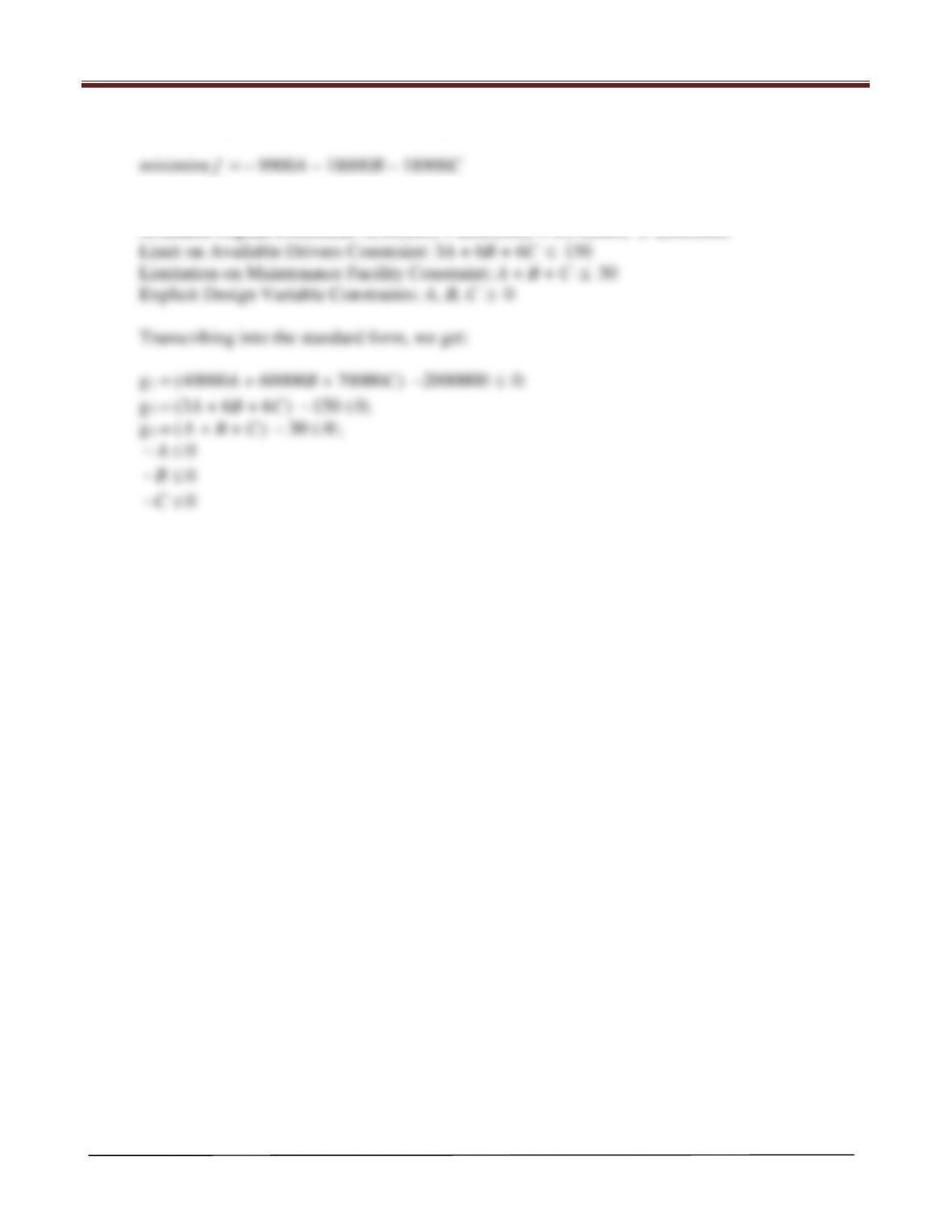
Step 3: Definition of Design Variables
Chapter 2 Optimum Design Problem Formulation
Arora, Introduction to Optimum Design, 4e
2-29
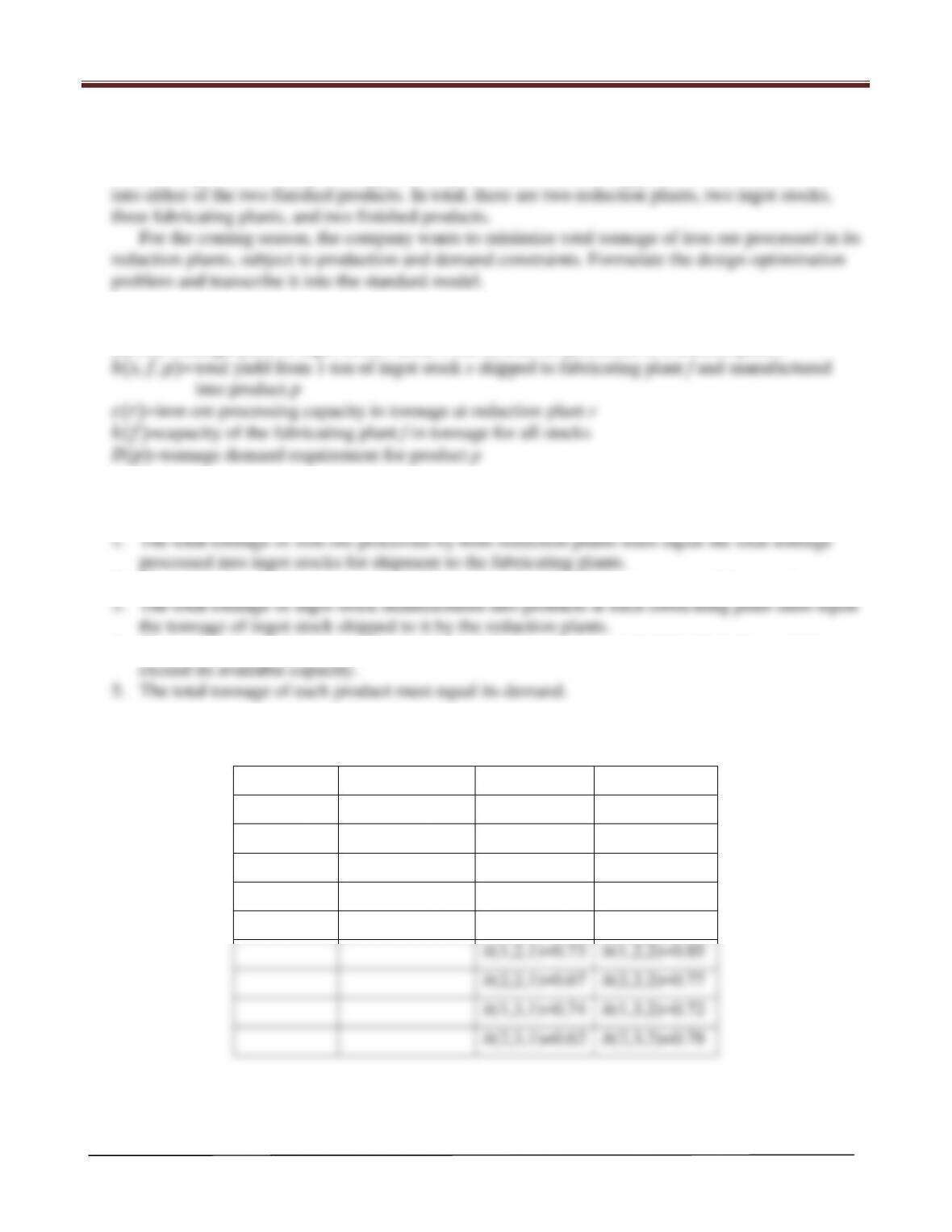
Transcribing into the standard form, we get:
Step 5: Formulation of Constraints
Available Capital Constraint: A(40,000) + B(60,000) + C(70,000)
≤
2,000,000
≤
≤
≥
Chapter 2 Optimum Design Problem Formulation
Arora, Introduction to Optimum Design, 4e
2-30
2.21*_______________________________________________________________________________
A large steel corporation has two iron ore reduction plants. Each plant processes iron ore into two
different ingot stocks. They are shipped to any of the three fabricating plants where they are made
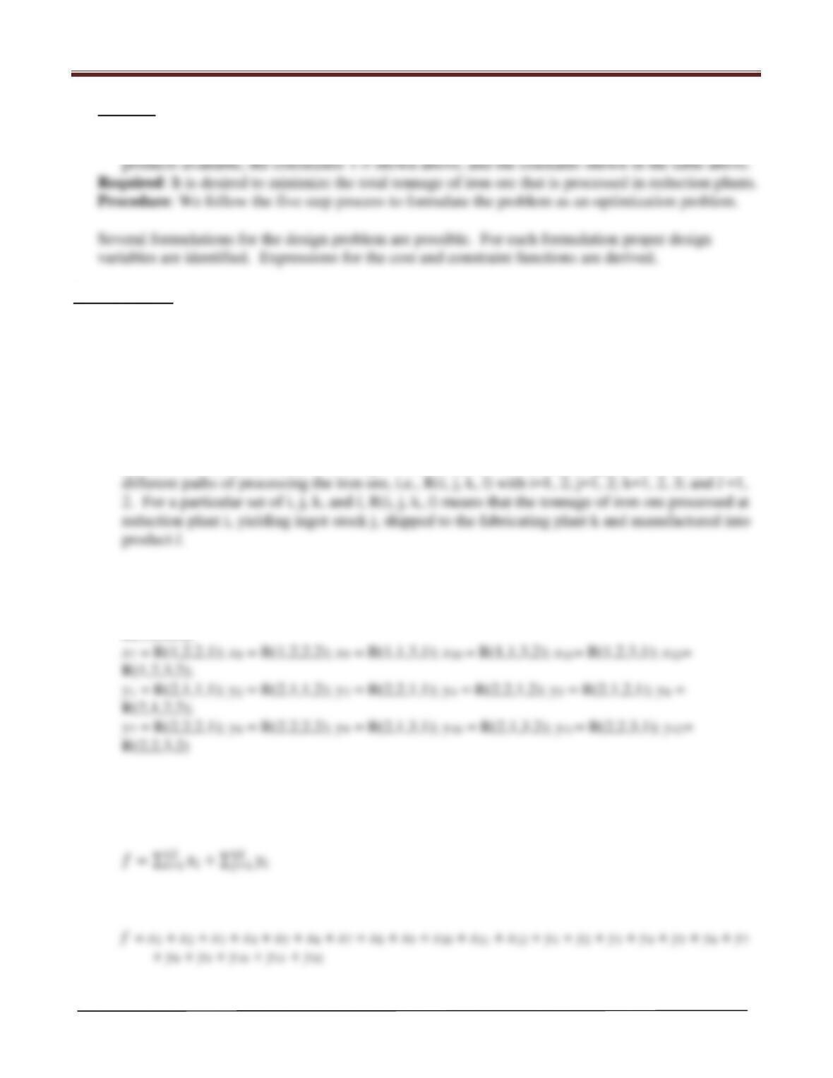
Nomenclature
(,)=tonnage yield of ingot stock s from 1 ton of iron ore processed at reduction plant r
Production and demand constraints
2. The total tonnage of iron ore processed by each reduction plant cannot exceed its capacity.
4. The total tonnage of ingot stock manufactured into products at each fabrication plant cannot
Constants for the problem
a(1,1)=0.39
c(1)=1,200,000
k(1)=190,000
D(1)=330,000
a(1,2)=0.46
c(2)=1,000,0 00
k(2)=240,000
D(2)=125,000
a(2,1)=0.44
k(3)=290,000
a(2,2)=0.48
b(1,1,1)=0.79
b(1,1,2)=0.84
b(2,1,1)=0.68
b(2,1,2)=0.81
b(1,2,1)=0.73
b(1,2,2)=0.85
b(2,2,1)=0.67
b(2,2,2)=0.77
b(1,3,1)=0.74
b(1,3,2)=0.72
b(2,3,1)=0.62
b(2,3,2)=0.78
Chapter 2 Optimum Design Problem Formulation
Arora, Introduction to Optimum Design, 4e
2-31
Solution
Given: The maximum number of reduction plants, ingot stocks, fabricating plants, and finished
Formulation 1:
Step 1: Problem Statement
Shown above
Step 2: Data and Information Collection
Shown above
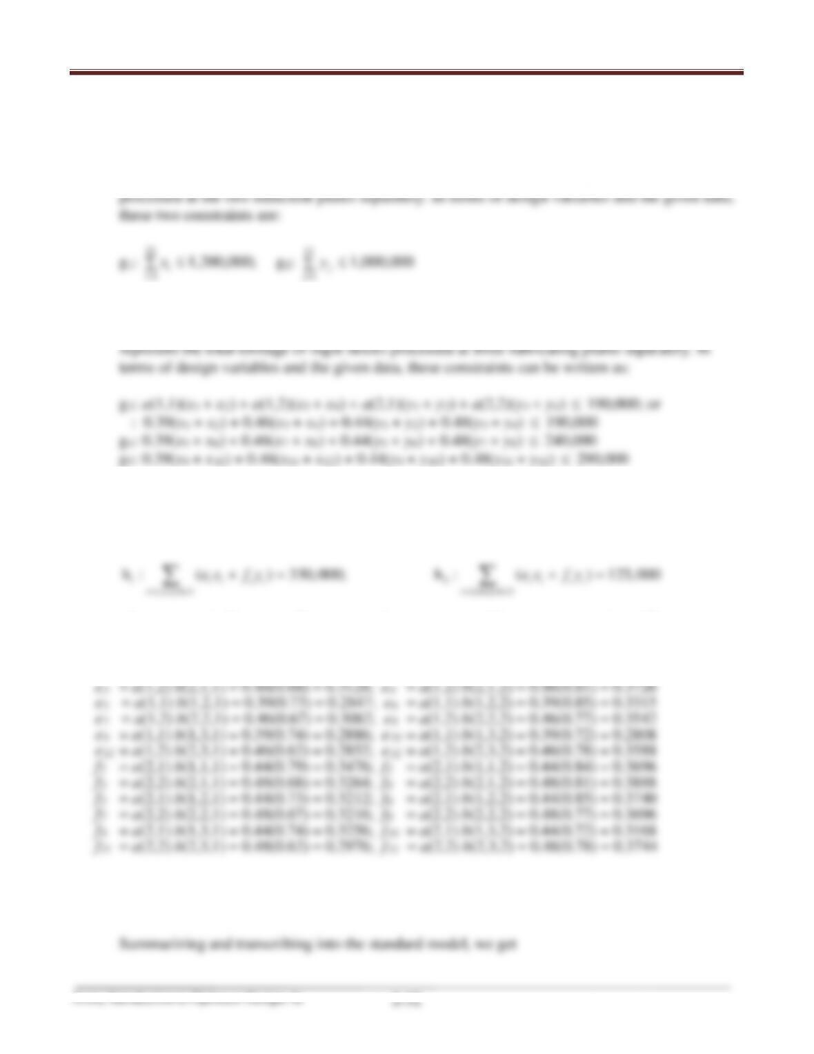
Step 3: Definition of Design Variables
For this formulation, twenty-four design variables are chosen which designate the twenty–four
For simplicity of the following derivation, let
x1 = R(1,1,1,1); x2 = R(1,1,1,2); x3 = R(1,2,1,1); x4 = R(1,2,1,2); x5 = R(1,1,2,1); x6 =
R(1,1,2,2);
Step 4: Optimization Criterion
Optimization criterion is to minimize total tonnage of iron ore processed at the reduction plants,
and the cost function is defined as
Summarizing and transcribing into the standard model, we get
Chapter 2 Optimum Design Problem Formulation
Step 5: Formulation of Constraints
(1) The total tonnage of iron ore processed by each reduction plant cannot exceed its capacity,
i.e., RP1
≤
c(1); RP2
≤
c(2) where RP1 and RP2 represent the total tonnage of iron ore
1=
i
i
1=
j
j
(2) The total tonnage of ingot stocks manufactured into products at each fabricating plant cannot
exceed its available capacity, i.e., F1 ≤ k(1); F2 ≤ k(2); F3 ≤ k(3) where F1, F2 and F3
≤
≤
≤
(3) The total tonnage of each product p1 and p2 respectively, must be equal to its demand, i.e.,
p1 = D(1); p2 = D(2) In terms of the design variables and the given data, the two constraints
are written as:
where
i
e
‘s and
i
f
‘s are coefficients transferring tonnage of iron ore into products. These
coefficients are given as:
e1 = a(1,1) b(1,1,1) = 0.39(0.79) = 0.3081; e2 = a(1,1) b(1,1,2) = 0.39(0.84) = 0.3276
(4) There are constraints requiring that both the reduction plants and fabricating plants do not
have any inventory of their own. These constraints have been satisfied automatically since the
twenty-four design variables (paths) are chosen which satisfy these conditions.