Chapter 2 Optimum Design Problem Formulation
Arora, Introduction to Optimum Design, 4e
2-33
h1 = 0.3081 x1 + 0.3128 x3 + 0.2847 x5 + 0.3082 x7 + 0.2886 x9 + 0.2852 x11 + 0.3476 y1 + 0.3264
y3 + 0.3212 y5 + 0.3216 y7 + 0.3256 y9 + 0.2976 y11 – 330,000 = 0
i
i
Formulation 2:
Step 1: Problem Statement
Shown above
Step 2: Data and Information Collection
Shown above
Step 3: Definition of Design Variables
The design variables are chosen as follows:
x1 : total tonnage of iron ore processed by plant 1;
x2 : total tonnage of iron ore processed by plant 2
x13 : tonnage of ingot stock 1 shipped to fabricating plant 3 to yield product 1
x14 : tonnage of ingot stock 1 shipped to fabricating plant 3 to yield product 2
x15 : tonnage of ingot stock 2 shipped to fabricating plant 1 to yield product 1
x16 : tonnage of ingot stock 2 shipped to fabricating plant 1 to yield product 2
x17 : tonnage of ingot stock 2 shipped to fabricating plant 2 to yield product 1
Step 4: Optimization Criterion
The cost function is defined as
Chapter 2 Optimum Design Problem Formulation
Arora, Introduction to Optimum Design, 4e
2-34
minimize f = x1 + x2
which is already in the standard form
Step 5: Formulation of Constraints
(1) The first constraint, total tonnage into each reduction plant must be equal to the tonnage
processed into ingot stocks for shipment, implies that there will be no stock piling at the
(2) The second constraint requires that the iron ore processed by each reduction plant should not
(3) The third constraint states that there is no stock piling at the fabricating plants. By the
definition of design variables, these are:
(4) The fourth constraint is on the maximum capacity of ingot stocks at each fabricating plant:
(5) The fifth constraint states that the total tonnage of each product must be equal to its demand:
In the standard form, the constraints become
Chapter 2 Optimum Design Problem Formulation
Arora, Introduction to Optimum Design, 4e
2-35
g3 = x9 + x10 + x15 + x16 – 190,000
≤
0
g4 = x11 + x12 + x17 + x18 – 240,000
≤
0;
g5 = x13 + x14 + x19 + x20 – 290,000
≤
0;
– xi
≤
0, i = 1 to 20
Chapter 2 Optimum Design Problem Formulation
2.22_____________________________________________________________________________
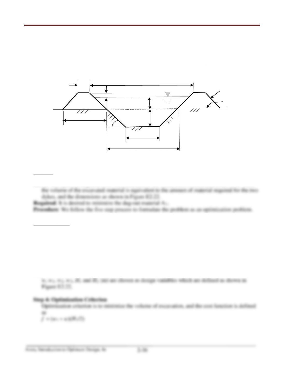
Optimization of water canal. Design a water canal having a cross–sectional area of 150 m2. Least
construction costs occur when the volume of the excavated material equals the amount of material
required for the dykes, i.e., 1=2 (see Figure E2.22). Formulate the problem to minimize the dug–
out material A1. Transcribe the problem into the standard design optimization model (created by
V.K.Goel).
FIGURE E2.22 Cross section of a canal.
Solution
Given: The specific, required cross–sectional area of the canal, least construction costs occur when
Formulation 1:
Step 1: Problem Statement
Shown above
Step 2: Data and Information Collection
Shown above
Step 3: Definition of Design Variables
Step 5: Formulation of Constraints
2m
1m
A
1
A
2
/2
A
2
/2
Dyke
Ground Level
w2
w
w1
w
3
H2
H1
θ
Chapter 2 Optimum Design Problem Formulation
Arora, Introduction to Optimum Design, 4e
2-37
The design variables are not independent; they are related as follows:
( ) ( ) ( )
1 2 31
2 22 2
ww w w w
− −−
So we get two more constraints from these relationships, as
1 31
ww w w
−−
All the design variables must also be nonnegative:
1
2
3
1
2
Formulation 2:
Step 1: Problem Statement
Shown above
Step 2: Data and Information Collection
Shown above
Step 3: Definition of Design Variables
w1, H1, H2 (m), and s (unitless) are chosen as design variables which are defined below in
12
31
2
2
2 ( 1)
2
ww s
H
ws
= +
+
= +
Step 4: Optimization Criterion
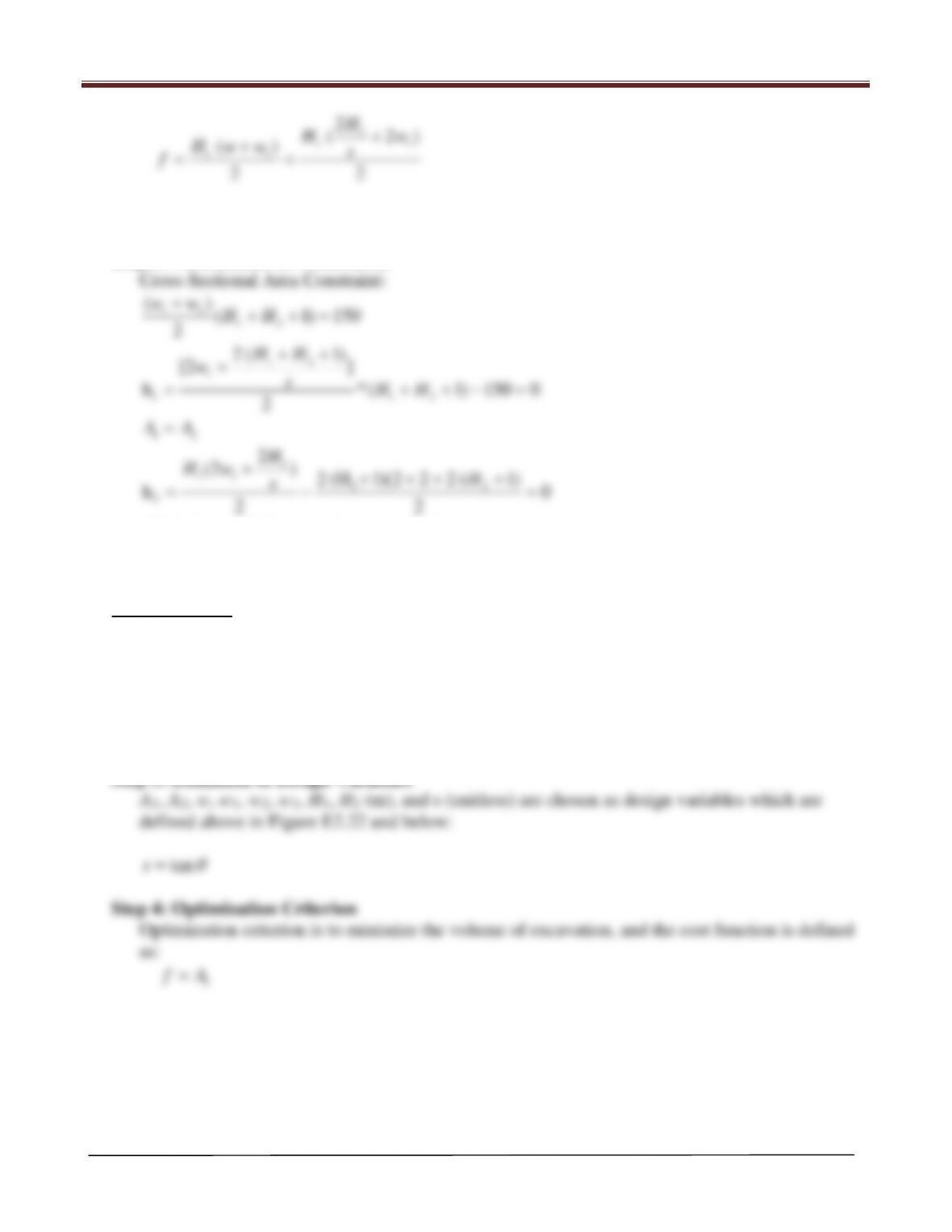
Optimization criterion is to minimize the volume of excavation, and the cost function is defined
as:
Chapter 2 Optimum Design Problem Formulation
Arora, Introduction to Optimum Design, 4e
2-38
1
11
11
2
( 2)
()
22
H
Hw
Hww s
f
+
+
= =
Step 5: Formulation of Constraints
Chapter 2 Optimum Design Problem Formulation
Step 5: Formulation of Constraints
Cross–Sectional Area Constraint:
13
12
13
1 12
12
12
1
22
2
12 2 2
2
1 2 12
1 2 31
12
3
12
11
4
1
()
( 1) 150
2
()
h ( 1) 150 0
2
( )H
2
2 (2 ) (H 1)
2
( ) H 2 (2 ) (H 1)
h0
22
2 2 (H 1) 2 ( 1)
( ) ( 2) ( )
2 2 (H 1)
h0
( ) ( 2)
2 2(
h()
wwHH
wwHH
AA
ww
A
w
A
ww w
H HH
sww w w w
H
ww w
H HH
ww
++ +=
+
= + +− =
=
+
=
++
=
+ ++
=−=
+ ++
= = =
−− −
+
=−=
−−
+
= −
−
2
31
2 12
5
2 31
1) 0
()
2 (H 1) 2 ( 1)
h0
( 2) ( )
All design variables 0
ww
HH
w ww
+=
−
+ ++
=−=
−−
≥
Arora, Introduction to Optimum Design, 4e
2-40
2.23________________________________________________________________________________
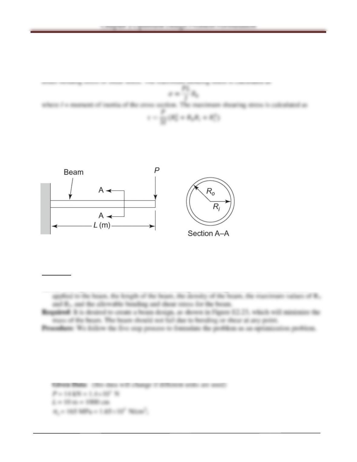
A cantilever beam is subjected to the point load P (kN), as shown in Fig. E2.23. The maximum
bending moment in the beam is PL (kN
⋅
m) and the maximum shear is P (kN). Formulate the
minimum mass design problem using a hollow circular cross section. The material should not fail
=
3(
Transcribe the problem into the standard design optimization model (also use 0≤ 40.0 cm,
≤40.0 cm). Use the following data: P = 14 kN ; L = 10 m; mass density, ρ=7850 kg/m3,
allowable bending stress, σa= 165 MPa, Allowable shear stress, τa =50 MPa.
FIGURE E2.23 Cantilever beam.
Solution
Given: The equations to calculate maximum bending and shearing stress in the beam, the force
Step 1: Problem Statement
Shown above
Step 2: Data and Information Collection
Using kg, N and cm as units
b
Chapter 2 Optimum Design Problem Formulation
Arora, Introduction to Optimum Design, 4e
2-41
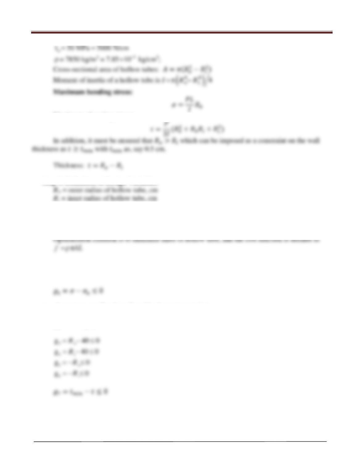
Maximum shearing stress:
2+0+
2)
Step 3: Definition of Design Variables
FORMULATION 1: Using Intermediate Variables
Step 4: Optimization Criterion
Step 5: Formulation of Constraints
g1 : bending stress should be smaller than the allowable bending stress; ≤
g2 : shear stress smaller than allowable shear stress: ≤
2= − ≤0
FORMULATION 2: Using only Design Variables
Chapter 2 Optimum Design Problem Formulation
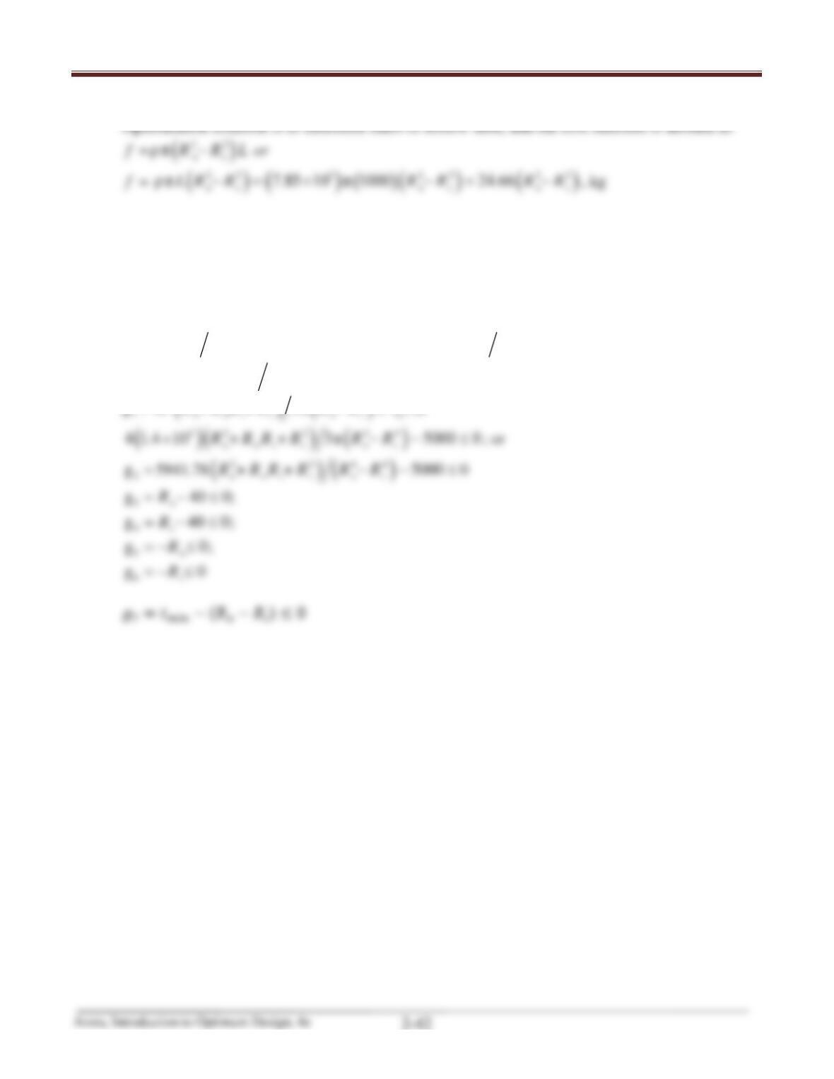
Step 4: Optimization Criterion
oi oi oi
Step 5: Formulation of Constraints
g1 : bending stress should be smaller than the allowable bending stress
g2 : shear stress smaller than allowable shear stress
Using the standard form, we get
g1 :
( )
44
o oi
4Pl R R Rπ− ≤
b
σ
; or
( ) ( ) ( )
4 3 44 4
o oi
4 1.4 10 10 1.65 10 0;R RR× π− − ×≤
or
g1
=
1.7825
7
10×
( )
44 4
o oi1.65 10R RR− − ×≤
0
g2 :
( ) ( )
2 2 44
o oi i o i
4++3
a
PR RR R R Rπ − ≤τ
; or
4 2 2 44
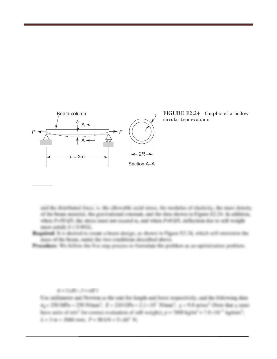
Chapter 2 Optimum Design Problem Formulation
Arora, Introduction to Optimum Design, 4e
2-43
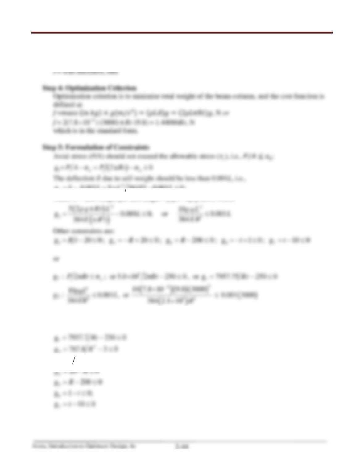
2.24________________________________________________________________________________
Design a hollow circular beam-column, shown in Figure E2.24, for two conditions: When the axial
tensile load P=50 (kN), the axial stress σ must not exceed an allowable value σa, and when P=0,
deflection δ due to self-weight should satisfy the limit δ ≤ 0.001L. The limits for dimensions are:
thickness t=0.10 to 1.0 cm, mean radius R=2.0 to 20.0 cm, and R/t ≤ 20 (AISC, 2005). Formulate the
minimum-weight design problem and transcribe it into the standard form. Use the following data:
deflection δ=5wL4/384EI; w=self–weight force/length (N/m); σa=250 MPa; modulus of elasticity
E=210 GPa; mass density of beam material ρ=7800 kg/m3; axial stress under load P, σ=P/A;
gravitational constant g=9.80 m/s2; cross–sectional area A = 2πRt (m2); moment of inertia of beam
cross–section I=πR3t (m4). Use Newton (N) and millimeters (mm) as units in the formulation.
Solution
Given: The maximum and minimum dimensions of t and R and the maximum ratio for R/t, the
equations to calculate displacement, δ, axial stress, σ, cross–sectional area, moment of inertia,
Step 1: Problem Statement
Shown above
Step 2: Data and Information Collection
Assuming that the wall is thin (R >> t), the cross-sectional area and moment of inertia are:
3
Chapter 2 Optimum Design Problem Formulation
Step 3: Definition of Design Variables
R = mean radius of the section, mm
4
2
g 0.001 5 384 0.001 0L wL EI L=δ− = − ≤
;
where w = self-weight per unit length =
2gA g R tρ =ρπ
, N/mm
g 20 0Rt= −≤
( )
44
52 10
g Rt L gL
ρπ ρ
3
7
( )
252
384 384 2.1 10
ER R
×
Summarizing the constraints and rewriting in standard form, we get
1
2
2
g 767.8 3 0R= −≤
3
g 20 0Rt= −≤
4
g 20 0R= −≤
7