Arora, Introduction to Optimum Design, 3e 14-1
CHAPTER
14
Practical Applications of Optimization
Note: In all the numerical results presented with IDESIGN (a program based on the SQP method), very
severe convergence criteria are used to obtain a precise solution (maximum constraint violation ≤ 0.0001
and convergence parameter ≤ 0.0001). Relaxed convergence criteria can give near optimum solutions in
fewer iterations.
14.1 ________________________________________________________________________________
Using the data given in Exercise 3.34 (l = 500mm), the problem is stated as follows after
normalizing the constraints:
Find x1 = outer diameter of the shaft (mm) and x2 = ratio of inner to outer diameters to minimize:
mass f (x1, x2) = (3.08269 × 10−3) x
22
12
(1 )x−
, kg;
34
12
g3 = 1 − 2.08623×10-3 x
3
12
(1 )x−
2.5 ≤ 0.
The problem is solved using the IDESIGN program where explicit design variable bound
2
14.2 ________________________________________________________________________________
Using the data given in Exercise 3.35 ( l = 500mm), the problem is stated as follows after
normalizing the constraints:
Find x1 = outside diameter of the shaft (mm), x2 = inside diameter of the shaft(mm) to minimize the
mass f (x1, x2) = (3.08269 ×10⁻³) (x
2
1
− x
2
2
), kg
subject to g1 = (1.852×105) x1/(x
4
1
− x
4
2
) −1 ≤ 0;
g2 = 1.82378×10⁷/(x
4
1
− x
4
2
) − 1 ≤ 0
3
2.5 ≤ 0;
Chapter 14 Practical Applications of Optimization
Arora, Introduction to Optimum Design, 4e
14-3
14.3 ________________________________________________________________________________
Using the data given in Exercise 3.36 (l = 500mm), the problem is stated as follows after
normalizing the constraints:
Find x1 = mean radius (mm) and x2 = wall thickness (mm) to minimize the mass
3
3
Starting from the point x1 = 50 mm, x2 = 2 mm, the optimum solution is obtained in 4 iterations
with convergence criteria as 0.0001 using the SQP algorithm:
*
1
*
2
*
*
*
2
Chapter 14 Practical Applications of Optimization
Arora, Introduction to Optimum Design, 4e
14-4
14.5 ________________________________________________________________________________
Using the data and expressions given in Exercise 3.51, the problem is stated as follows after
normalizing the constraints:
Find R = mean radius (cm) and t = wall thickness (cm) to minimize the mass of the water tower
support column: f (R, t) = 153.717 Rt
6
4.04488 10
×
5257.21(2 )
+
Rt
10
(1.6492 10 )(2 )
Rt
×+
14.6 ________________________________________________________________________________
Using the data and expressions given in Exercise 3.52, the problem is stated as follows after
normalizing the constraints:
Find do = outer diameter (cm) and di = inner diameter (cm) to minimize the mass of the flag pole:
f = 6.12611(d
2
o
− d
2
i
), kg;
subject to g1 = 8642.61do / (d
4
o
− d
4
i
) –1 ≤ 0; g2 = 8.14874(d
2
o
+ dodi+ d
2
i
)/(d
4
o
− d
4
i
) −1 ≤ 0;
4
o
i
4
Chapter 14 Practical Applications of Optimization
Arora, Introduction to Optimum Design, 4e
14-5
14.7 ________________________________________________________________________________
Using the data and expressions given in Exercise 3.53, the problem is formulated as follows after
normalizing the constraints: find do = outer diameter (mm) and t = wall thickness (mm) to
minimize the weight of the sign support: f = 5.02655t(do− t), N
9
1.687973 10
×
7
(4.0976487 10 )
o
d
×
17
(1.435461 10 )
o
d
×
14.8 ________________________________________________________________________________
Using the data and expressions given in Exercise 3.54, the problem is formulated as follows after
normalizing the constraints:
Find H = height of the tripod and D = diameter of the cross–section to minimize the mass of the
Chapter 14 Practical Applications of Optimization
Arora, Introduction to Optimum Design, 4e
14-6
14.9 ________________________________________________________________________________
Problem formulation: Minimize f = bh;
subject to g1 = 1.0 − [3gkEI/(3WEI + kWL3)]1/2/8.0 ≤ 0, where I = bh3/12,
14.10 ______________________________________________________________________________
Formulation: Units of N and cm are used
a − 1.0 ≤ 0, where M = PLsin
L = 150,
θ
= 45°,
σ
a = 10000, c = x2 + x4/2, I = [x1(2x2+ x4)3 − (x1− x3) x
3
4
] / 12, A = 2x1x2 + x3x4 ;
<shear stress> g2 = (VQ / I x3)/
τ
a − 1.0 ≤ 0, where V = Psin
θ
, Q = x1x2(x2+ x4)/2 + x3x
2
4
/8,
τ
a =
3
3
1
3
Solution: Program IDESIGN (SQP algorithm) is used.
Initial design; x1= 60, x2= 0.9, x3= 0.9, x4= 14;
*
1
*
2
*
3
*
4
*
number of iterations: 7, active constraints (Lagrange multipliers): g1(15502.0), g2(805.224), upper
limit of x2(154.797), upper limit of x4(14641.4).
*
Chapter 14 Practical Applications of Optimization
Arora, Introduction to Optimum Design, 4e
14-7
14.11 _______________________________________________________________________________
Formulation:
1ii
i
=
1i
i
=
3. Constraints (18 stress constraints):
gj =
σ
1j /5000 − 1.0 ≤ 0, j = 1,2,3; g3+j = − σ1j /5000 − 1.0 ≤ 0, j = 1,2,3;
*
1
b
*
2
= A2 = 2.0458, b
*
3
= A3 = 2.9271 in2, b
*
4
= x1 = − 4.6716, b
*
5
= x2 = 8.9181, b
*
6
= x3 = 4.6716 in,
*
f
= 75.3782 in3 ; active constraints (Lagrange multipliers): g3(27.411), g7(4.86191), g11(0.0),
g13(20.5489), g17(22.5562).
14.12 _______________________________________________________________________________
Formulation: Minimize f = (x2 − x3)2;
subject to h1 =
φ
2x1(x1 − x2 + x3)/x2 x3 − 1 = 0, h2 = 1.0 − x2(1 − x1+ x2)/
φ
3x1 = 0, and design bounds
1.0E−10 ≤ x1, x2, x3 ≤ 1000.0
Solution for
φ
= 2 ; Program used: IDESIGN (SQP algorithm; 8 iterations), x(0) = (1, 1, 1).
f
*
1
*
2
*
3
*
multipliers): h1(− 0.007119), h2(0.003528)
Solution for φ = 21/3 ; Program used: IDESIGN (SQP algorithm; 8 iterations), x(0) = (1, 1, 1).
f
*
1
*
2
*
3
*
multipliers); h1(− 5.47×10− 6), h2(1.6236×10− 6).
Chapter 14 Practical Applications of Optimization
Arora, Introduction to Optimum Design, 4e
14-8
14.13 _______________________________________________________________________________
Formulation: units of N, kg, and cm are used.
1. Design variables: x1 = outside diameter of the pole at the base, x2 = outside diameter of the
2. Cost function: f =
ρ
∫
0
H
A(x)dx =
ρπ
Hx3(x1/2 + x2/2 − x3), where A(x) =
π
x3[d(x) − x3] = cross–
3. Constraints: <bending stress> g1 =
σ
(x)/
σ
b − 1.0 ≤ 0, where
σ
(x) = M(x) d(x)/2I(x), M(x) =
bending moment at x = P(H − x) + w(H − x)2/2, I(x) = moment of inertia of the cross-section at x =
π
[{d(x)}4 − {d(x) − 2x3}4]/64 = A(x)[{d(x)}2 + {d(x) − 2x3}2]/16. Since the constraint g1 depends
on the distance x, we impose it at x = 0 and five other points that give local maximum of g1;
<shearing stress> g7 =
τ
(x)/
τ
s − 1.0 ≤ 0, where
τ
(x) = S(x)[d2(x) + d(x){d(x) − 2x3} + d(x) − 2x3}2] /
24I(x)x3, S(x) = shear force at x = P + w(H − x). This constraint is also a function of x and it is
imposed at x = 0 and x = H;
<deflection> g9 =
δ
/10 − 1.0 ≤ 0, where
δ
= deflection at the top = ∫
0
H
[M(x)(H − x)/EI(x)]dx.
δ
is
evaluated numerically using the Gaussian quadrature for the numerical integration;
<ratio> g10 = (x1 − x3)/60x3 − 1.0 ≤ 0,
g11 = (x2 − x3) /60x3 − 1.0 ≤ 0;
<design bounds> 5 ≤ x1 ≤ 50, 5 ≤ x2 ≤ 50, 0.5 ≤ x3 ≤ 2.
Solution: Program IDESIGN (SQP algorithm) is used. Initial design: x1 = 30.0, x2 = 30.0,
*
*
*
*
Chapter 14 Practical Applications of Optimization
3
2
*
14.14 _______________________________________________________________________________
Formulation: units of N, kg, and mm are used.
1. Definition of variables; x1 = outer diameter of the pole at the base (x = 0), x2 = outside
diameter of the pole at the top (x = H ), x3 = thickness, x = distance from the base (0 ≤ x ≤ H + h),
A(x) = cross–sectional area of the pole =
π
x3[x1− x(x1− x2)/H − x3], d(x) = outer diameter = x1 −
x(x1− x2)/H, I(x) = moment of inertia of the cross-section = A(x)[2x2(x1− x2)2/H2 +
x(x1− x2)(x3− x1) /H + 2x
2
1
− 4x1x3 + 4x
2
3
]/16,
δ
(x) = horizontal deflection, M(x) = bending moment
of the pole = F(H + h/2 − x) + W [
δ
(H) −
δ
(x)], F = wind force = pbh , W = weight of sign = wbh,
fa(x) = axial stress = W/A(x), fb(x) = bending stress = M(x) d(x)/2I(x),
σ
a = allowable axial stress
(approximated) = (12/23)Pcre /Ae, Pcre = effective critical buckling load (approximated as linear
combination of Pcr at x = 0 and Pcr at x = H ) = c1
π
2EI(0)/4H2 + c2
π
2EI(H )/4H2, (in the current
computation, c1 = c2 = 0.5 are used), Ae = effective cross–sectional area (approximated as linear
combination of A(0) and A(H)) = c3 A(0) + c4 A(H), where c3 = 1 and c4 = 0 are assumed.
2. Cost function:
H
Arora, Introduction to Optimum Design, 4e
14-10
14.15 _______________________________________________________________________________
Formulation: x1 = outer width of the pole at the base, x2 = outer width of the pole at the top, x3 =
thickness, d(x) = outer width of the pole at the distance x from the base = x1 − x(x1− x2)/H; Note
that d(0) = x1 and d(H) = x2. A(x) = cross–sectional area at x = 4x3[x1− x(x1− x2)/H − x3]; Note that
14.13),
g7 = S(x) Q(x)/2x3I(x)
τ
s − 1.0 ≤ 0 (2 constraints are imposed at x = 0 and x = H ), where Q(x)=
[d3(x) − {d(x) − 2x3}3]/8,
g9 =
δ
/10 − 1.0 ≤ 0,
g10 = (x1− x3)/60x3 − 1.0 ≤ 0,
g11 = (x2 − x3)/60x3 − 1.0 ≤ 0,
5 ≤ x1 ≤ 50, 5 ≤ x2 ≤ 50, 0.5 ≤ x3 ≤ 2.
Solution: Program IDESIGN (SQP algorithm) is used. Initial design: x1 = 30.0, x2 = 30.0, x3 = 1.0.
*
*
*
*
Chapter 14 Practical Applications of Optimization
14.16 _______________________________________________________________________________
Formulation: Problem formulation is exactly the same as Exercise 14.14 except the definitions of
following variables and expressions. x1 = outer width of the hollow square at the base; x2 = outer
width of the hollow square at the top; x3 = thickness; d(x) = outer width of the hollow square at a
distance x from the base = x1 − x(x1− x2)/H; A(x) = d2(x) − [d(x) − 2x3]2;
I(x) = [d4(x) − (d(x) − 2x3)4]/12;
*
f
= cost function = 4
γ
Hx3(x1/2 + x2/2 − x3);
*
f
14.17 _______________________________________________________________________________
Case 1: ua = 25; f1 = 1.07301E−06, f2 = 1.83359E−02, f3 = 2.49977E+01, f4 = 0.10, NIT = 39,
14.18 _______________________________________________________________________________
Case 1: ua = 25; f 1 = 2.31697E−06, f 2 = 2.74712E−02, f 3 = 7.54602, f 4 = 0.10, NIT = 11, NCF
= 11, NGE = 62.
14.19 _______________________________________________________________________________
Case 1: ua = 25; f 1 = 1.11707E−06, f 2 = 1.52134E−02, f 3 = 19.8150, f 4 = 3.3052E−02, NIT =
14.20 _______________________________________________________________________________
14.21 _______________________________________________________________________________
Arora, Introduction to Optimum Design, 4e
14-12
14.22 _______________________________________________________________________________
14.23 _______________________________________________________________________________
14.24 _______________________________________________________________________________
14.25 _______________________________________________________________________________
89.
14.27 _______________________________________________________________________________
14.28 _______________________________________________________________________________
Chapter 14 Practical Applications of Optimization
Arora, Introduction to Optimum Design, 4e
14-13
14.29 _______________________________________________________________________________
Formulation: Use the artificial variable as a cost function; design variables: k = spring constant, c =
damping coefficient, A = artificial variable;
cost function: f = A;
Chapter 14 Practical Applications of Optimization
Section 14.8 Optimum Design of Tension Members
14.31 _____________________________________________________________________________
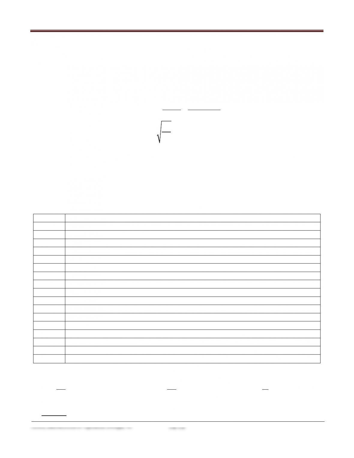
Solve the following problem using the Excel Solver:
Solve the W-shape optimization problem of Section 14.8 where a W14 shape is desired.
33
2 ( 2)
( ) ( 2)
212 12
g ff f w
ff f w
y
y
y
g
A bt d t t
tb d t t
I
I
rA
= +−
−
= +
=
Design variables for the W-shape optimization problem are defined as a vector
x = (d, bf, tf, tw)
The optimization function for the mass minimization problem is given as
12 , lbs/ft
g
fA
γ
=
TABLE E14.31
Notation
Data
Ag
Gross area of the section, in2
An
Net area (gross area less cross-sectional areas due to bolt holes), in2
Ae
Effective net area, Ae=UAn, in2
bf
Width of flange, in
d
Depth of section, in
Fy
Specified minimum yield stress, 50 ksi for A992 steel, ksi
Fu
Specified minimum ultimate stress, 65 ksi for A992 steel, ksi
L
Laterally supported length of member, in
Pn
Nominal axial strength, kips
Pa
Required strength, kips
ry
Least radius of gyration, in
tf
Thickness of flange, in
tw
Thickness of web, in
U
Shear lag coefficient: reduction coefficient for net area
x
Distance for plane of shear transfer to centroid of tension member cross section, in
Ωt
Factor of safety for tension, 1.67 and 2.00, for yielding and rupture, respectively
γ
Density of steel, 0.283 lb/in3
The constraints for the W-shape design problem are given as
; 0.6 , ; 0.5 , 300
ny nr
a ny y g a y g a nr u e a u e
t ty
PPL
P P FA P FA P P FA P FA r
≤ = →≤ ≤ = →≤ ≤
ΩΩ
Solution
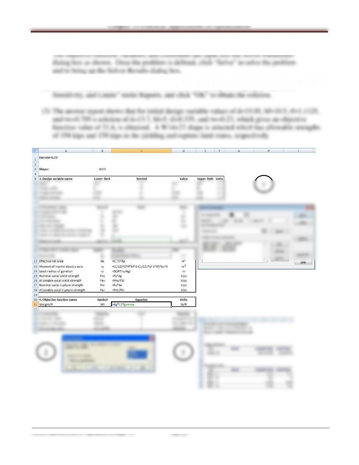
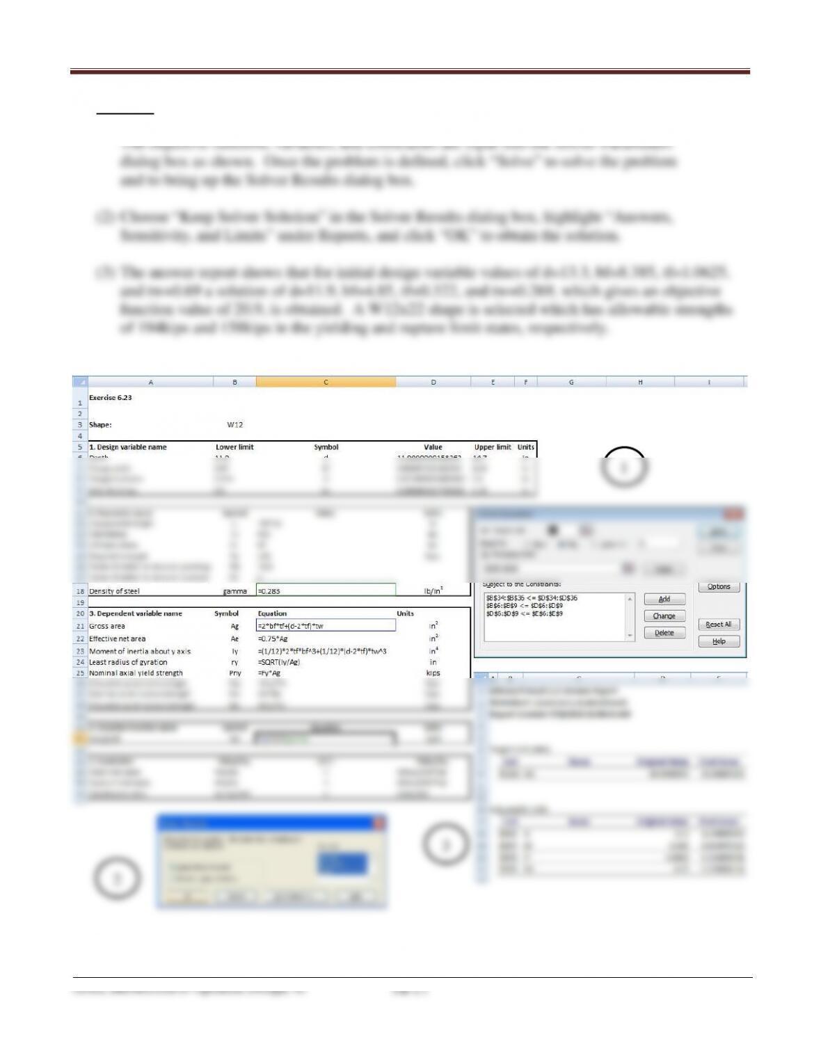
(1) One possible format for setting up the Excel worksheet for this problem is shown below.
(2) Choose “Keep Solver Solution” in the Solver Results dialog box, highlight “Answers,
3
1
2
Arora, Introduction to Optimum Design, 4e
14-16
14.32______________________________________________________________________________
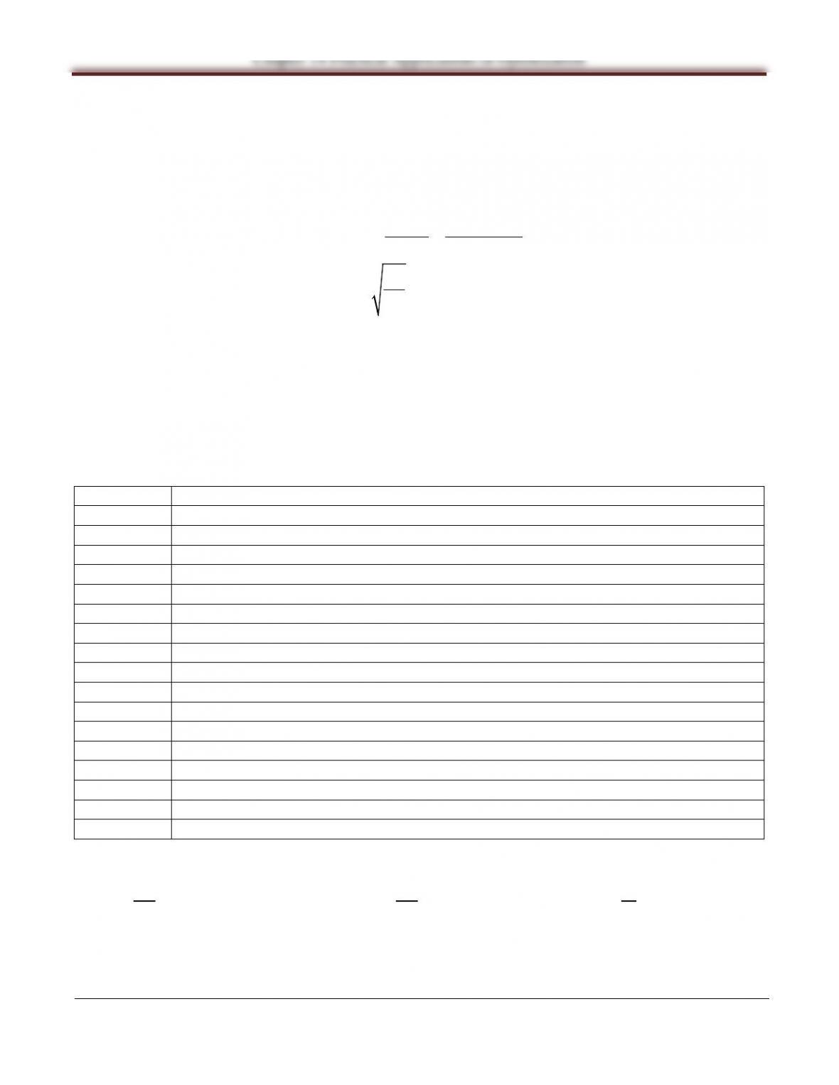
Solve the following problem using the Excel Solver:
Solve the W-shape optimization problem of Section 14.8 where a W12 shape is desired.
33
2 ( 2)
( ) ( 2)
212 12
g ff f w
ff f w
y
y
y
g
A bt d t t
tb d t t
I
I
rA
= +−
−
= +
=
Design variables for the W-shape optimization problem are defined as a vector
x = (d, bf, tf, tw)
The optimization function for the mass minimization problem is given as
12 , lbs/ft
g
fA
γ
=
TABLE E14.32
Notation
Data
Ag
Gross area of the section, in2
An
Net area (gross area less cross-sectional areas due to bolt holes), in2
Ae
Effective net area, Ae=UAn, in2
bf
Width of flange, in
d
Depth of section, in
Fy
Specified minimum yield stress, 50 ksi for A992 steel, ksi
Fu
Specified minimum ultimate stress, 65 ksi for A992 steel, ksi
L
Laterally supported length of member, in
Pn
Nominal axial strength, kips
Pa
Required strength, kips
ry
Least radius of gyration, in
tf
Thickness of flange, in
tw
Thickness of web, in
U
Shear lag coefficient: reduction coefficient for net area
x
Distance for plane of shear transfer to centroid of tension member cross section, in
Ωt
Factor of safety for tension, 1.67 and 2.00, for yielding and rupture, respectively
γ
Density of steel, 0.283 lb/in3
The constraints for the W-shape design problem are given as
; 0.6 , ; 0.5 , 300
ny nr
a ny y g a y g a nr u e a u e
t ty
PPL
P P FA P FA P P FA P FA r
≤ = →≤ ≤ = →≤ ≤
ΩΩ
Chapter 14 Practical Applications of Optimization
Solution
(1) One possible format for setting up the Excel worksheet for this problem is shown below.
3
2
1
Arora, Introduction to Optimum Design, 4e
14-18
14.33____________________________________________________________________________
Solve the following problem using the Excel Solver:
Solve the W-shape optimization problem of Section 14.8 where a W8 shape is desired, the required
strength Pa for the member is 200 kips, the length of the member is 13 ft, and the material is A992
Grade 50 steel.
33
2 ( 2)
( ) ( 2)
212 12
g ff f w
ff f w
y
y
y
g
A bt d t t
tb d t t
I
I
rA
= +−
−
= +
=
Design variables for the W-shape optimization problem are defined as a vector
x = (d, bf, tf, tw)
The optimization function for the mass minimization problem is given as
12 , lbs/ft
g
fA
γ
=
TABLE E14.33
Notation
Data
Ag
Gross area of the section, in2
An
Net area (gross area less cross-sectional areas due to bolt holes), in2
Ae
Effective net area, Ae=UAn, in2
bf
Width of flange, in
d
Depth of section, in
Fy
Specified minimum yield stress, 50 ksi for A992 steel, ksi
Fu
Specified minimum ultimate stress, 65 ksi for A992 steel, ksi
L
Laterally supported length of member, 156 in
Pn
Nominal axial strength, kips
Pa
Required strength, 200 kips
ry
Least radius of gyration, in
tf
Thickness of flange, in
tw
Thickness of web, in
U
Shear lag coefficient: reduction coefficient for net area
x
Distance for plane of shear transfer to centroid of tension member cross section, in
Ωt
Factor of safety for tension, 1.67 and 2.00, for yielding and rupture, respectively
γ
Density of steel, 0.283 lb/in3
The constraints for the W-shape design problem are given as
; 0.6 , ; 0.5 , 300
ny nr
a ny y g a y g a nr u e a u e
t ty
PPL
P P FA P FA P P FA P FA r
≤ = →≤ ≤ = →≤ ≤
ΩΩ
Chapter 14 Practical Applications of Optimization
Arora, Introduction to Optimum Design, 4e
14-19
Solution
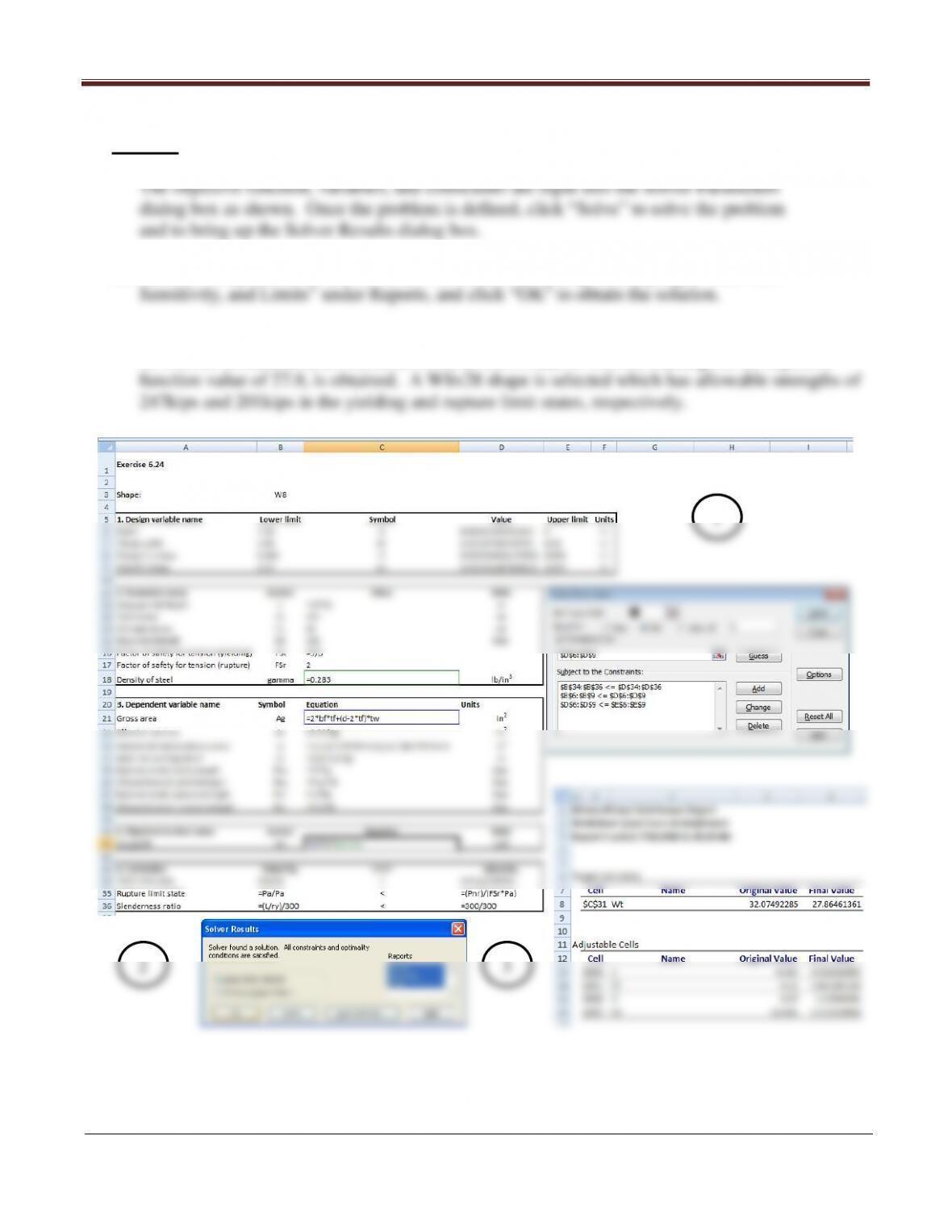
(1) One possible format for setting up the Excel worksheet for this problem is shown below.
(2) Choose “Keep Solver Solution” in the Solver Results dialog box, highlight “Answers,
(3) The answer report shows that for initial design variable values of d=8.465, bf=6.11, tf=0.57, and
tw=0.3385 a solution of d=8.083, bf=5.46, tf=0.539, and tw=0.331, which gives an objective
3
2
1
Chapter 14 Practical Applications of Optimization
14.34_____________________________________________________________________________
Solve the following problem using the Excel Solver:
Solve the W-shape optimization problem of Section 14.8 where a W10 shape is desired, the required
strength Pa for the member is 200 kips, the length of the member is 13 ft, and the material is A992
Grade 50 steel.
33
2 ( 2)
( ) ( 2)
212 12
g ff f w
ff f w
y
y
y
g
A bt d t t
tb d t t
I
I
rA
= +−
−
= +
=
Design variables for the W-shape optimization problem are defined as a vector
x = (d, bf, tf, tw)
The optimization function for the mass minimization problem is given as
12 , lbs/ft
g
fA
γ
=
TABLE E14.38
Notation
Data
Ag
Gross area of the section, in2
An
Net area (gross area less cross-sectional areas due to bolt holes), in2
Ae
Effective net area, Ae=UAn, in2
bf
Width of flange, in
d
Depth of section, in
Fy
Specified minimum yield stress, 50 ksi for A992 steel, ksi
Fu
Specified minimum ultimate stress, 65 ksi for A992 steel, ksi
L
Laterally supported length of member, 156 in
Pn
Nominal axial strength, kips
Pa
Required strength, 200 kips
ry
Least radius of gyration, in
tf
Thickness of flange, in
tw
Thickness of web, in
U
Shear lag coefficient: reduction coefficient for net area
x
Distance for plane of shear transfer to centroid of tension member cross section, in
Ωt
Factor of safety for tension, 1.67 and 2.00, for yielding and rupture, respectively
γ
Density of steel, 0.283 lb/in3
The constraints for the W-shape design problem are given as
; 0.6 , ; 0.5 , 300
ny nr
a ny y g a y g a nr u e a u e
t ty
PPL
P P FA P FA P P FA P FA r
≤ = →≤ ≤ = →≤ ≤
ΩΩ