Arora, Introduction to Optimum Design, 4e
14-40
14.41_______________________________________________________________________________
Continued.
3
2
1
Chapter 14 Practical Applications of Optimization
14.42_______________________________________________________________________________
Solve the following problem using the Excel Solver:
Solve the problem of Example 14.7 for a beam of span 10 ft. Assume noncompact shape and
inelastic LTB.
337.5 kip-ft, 37.5 kips
λ λ and λ λ
, 0.6 M
13.7 16.4, 5.0 16.0, 0.335 1.89, 0.23 1.18
aa
f pf w pw
pbr
n pa n
f fw
MV
LLL
M MM
db t t
= =
≤≤
<≤
≤≤
≤≤ ≤ ≤ ≤ ≤ ≤ ≤
Solution
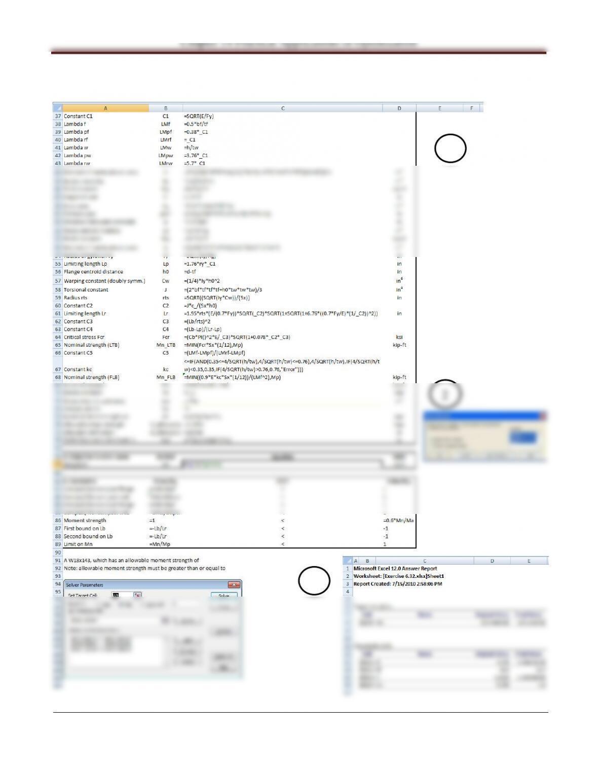
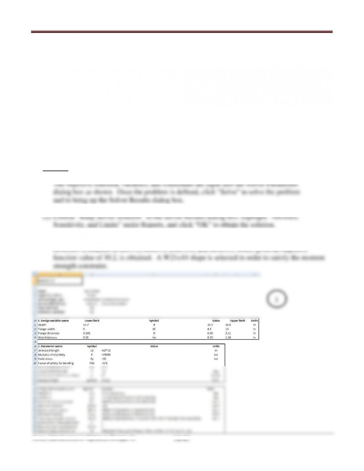
(1) One possible format for setting up the Excel worksheet for this problem is shown below.
(3) The answer report shows that for initial design variable values of d=19.6, bf=9, tf=1.223, and
Arora, Introduction to Optimum Design, 4e
14-42
14.42_______________________________________________________________________________
Continued.
3
2
1
Chapter 14 Practical Applications of Optimization
14.43_______________________________________________________________________________
Solve the following problem using the Excel Solver:
Solve the problem of Example 14.7 for a beam of span 40 ft. Assume noncompact shape and elastic
LTB.
337.5 kip-ft, 37.5 kips
λ λ and λ λ
, 0.6 M
13.7 16.4, 5.0 16.0, 0.335 1.89, 0.23 1.18
aa
f pf w pw
pbr
n pa n
f fw
MV
LLL
M MM
db t t
= =
≤≤
<≤
≤≤
≤≤ ≤ ≤ ≤ ≤ ≤ ≤
Solution
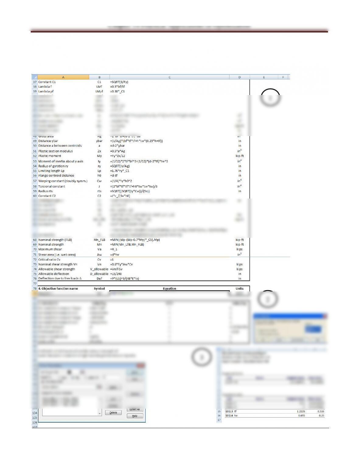
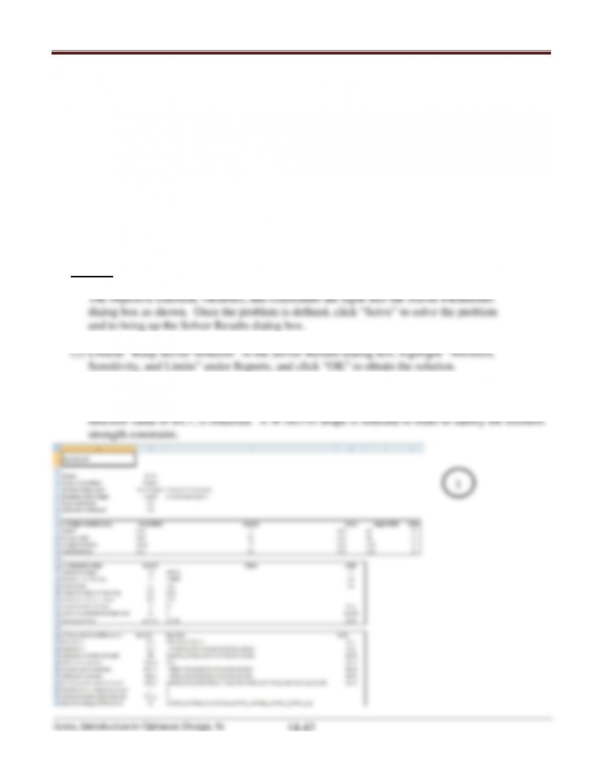
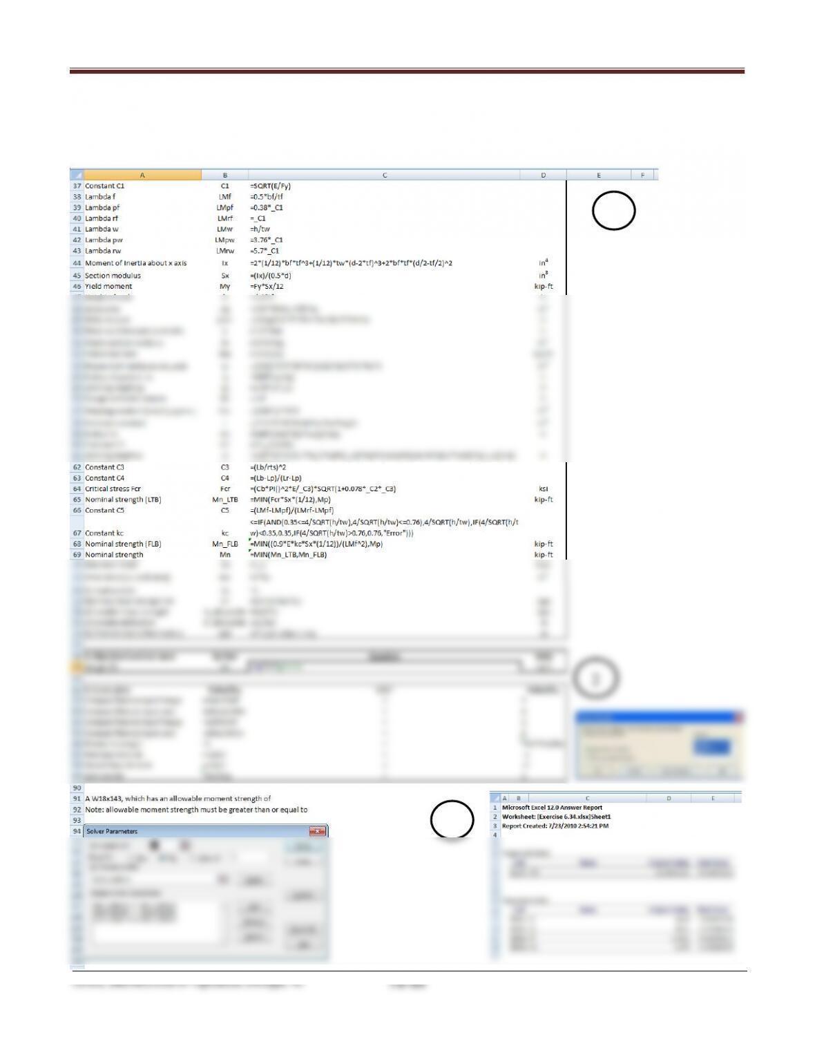
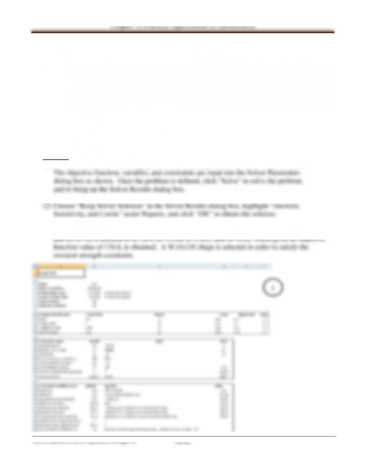
(1) One possible format for setting up the Excel worksheet for this problem is shown below.
(3) The answer report shows that for initial design variable values of d=24.08, bf=10.97, tf=2.24,
and tw=1.275 a solution of d=27.8, bf=17.44, tf=0.566, and tw=0.1944, which gives an objective
Chapter 14 Practical Applications of Optimization
14.43_______________________________________________________________________________
Continued
3
2
1
14.44_______________________________________________________________________________
Solve the following problem using the Excel Solver:
Design a cantilever beam of span 15 ft subjected to a dead load of 3 kips/ft and a point live load of
20 kips at the end. The material of the beam is A572 Grade 50 steel. Assume compact shape and
inelastic LTB.
337.5 kip-ft, 37.5 kips
λ λ and λ λ
, 0.6 M
13.7 16.4, 5.0 16.0, 0.335 1.89, 0.23 1.18
aa
f pf w pw
pbr
n pa n
f fw
MV
LLL
M MM
db t t
= =
≤≤
<≤
≤≤
≤≤ ≤ ≤ ≤ ≤ ≤ ≤
Solution
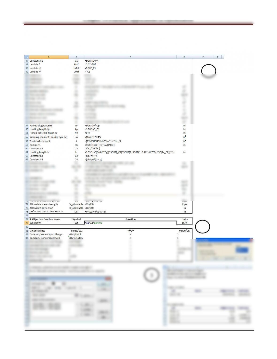
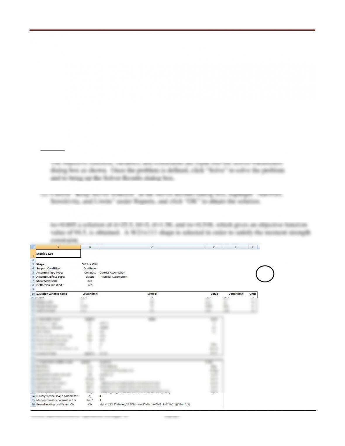
(1) One possible format for setting up the Excel worksheet for this problem is shown below.
(3) The answer report shows that for initial design variable values of d=15.05, bf=10.5, tf=1.1125,
Arora, Introduction to Optimum Design, 4e
14-46
14.44_______________________________________________________________________________
Continued.
3
2
1
Chapter 14 Practical Applications of Optimization
14.45_______________________________________________________________________________
Solve the following problem using the Excel Solver:
Design a cantilever beam of span 15 ft subjected to a dead load of 3 kips/ft and a point live load of
20 kips at the end. The material of the beam is A572 Grade 50 steel. Assume compact shape and
elastic LTB.
337.5 kip-ft, 37.5 kips
λ λ and λ λ
, 0.6 M
13.7 16.4, 5.0 16.0, 0.335 1.89, 0.23 1.18
aa
f pf w pw
pbr
n pa n
f fw
MV
LLL
M MM
db t t
= =
≤≤
<≤
≤≤
≤≤ ≤ ≤ ≤ ≤ ≤ ≤
Solution
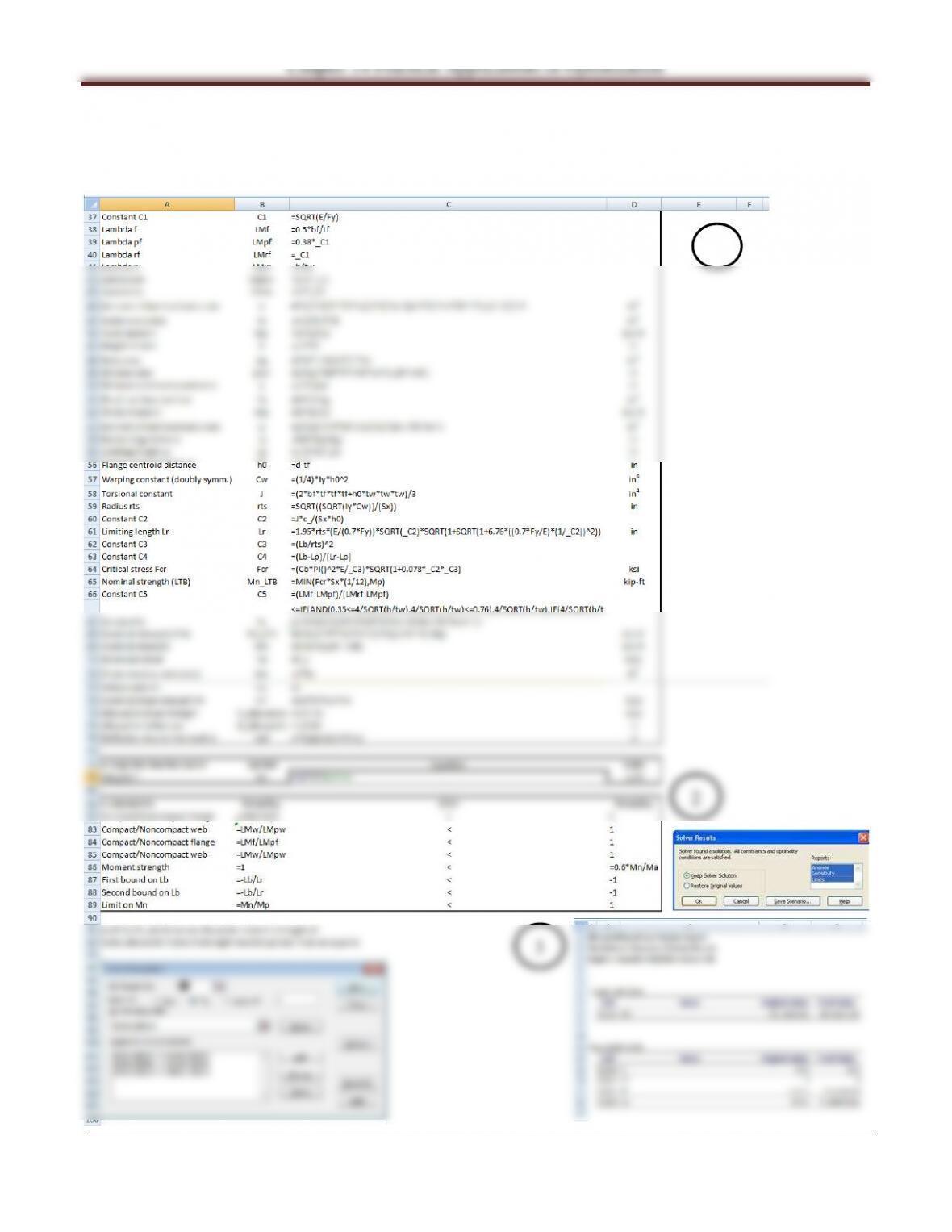
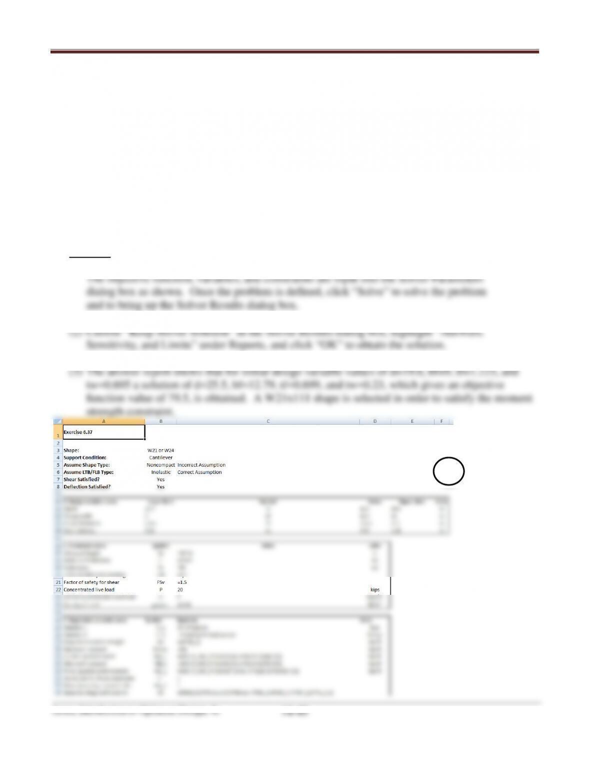
(1) One possible format for setting up the Excel worksheet for this problem is shown below.
(3) The answer report shows that for initial design variable values of d=19.6, bf=9, tf=1.223, and
1
Arora, Introduction to Optimum Design, 4e
14-48
14.45_______________________________________________________________________________
Continued.
3
2
1
Chapter 14 Practical Applications of Optimization
14.46_______________________________________________________________________________
Solve the following problem using the Excel Solver:
Design a cantilever beam of span 15ft subjected to a dead load of 3kips/ft and a point live load of
20kips at the end. The material of the beam is A572 Grade 50 steel. Assume noncompact shape and
inelastic LTB.
337.5 kip-ft, 37.5 kips
λ λ and λ λ
, 0.6 M
13.7 16.4, 5.0 16.0, 0.335 1.89, 0.23 1.18
aa
f pf w pw
pbr
n pa n
f fw
MV
LLL
M MM
db t t
= =
≤≤
<≤
≤≤
≤≤ ≤ ≤ ≤ ≤ ≤ ≤
Solution
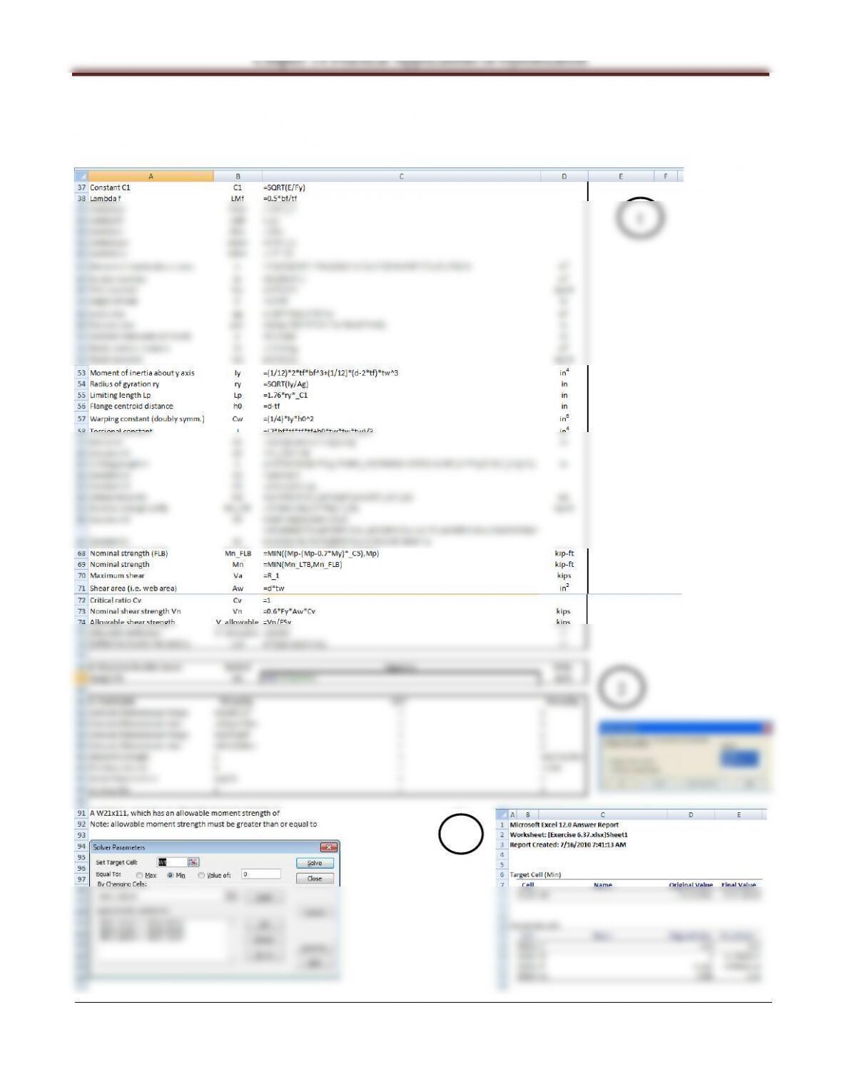
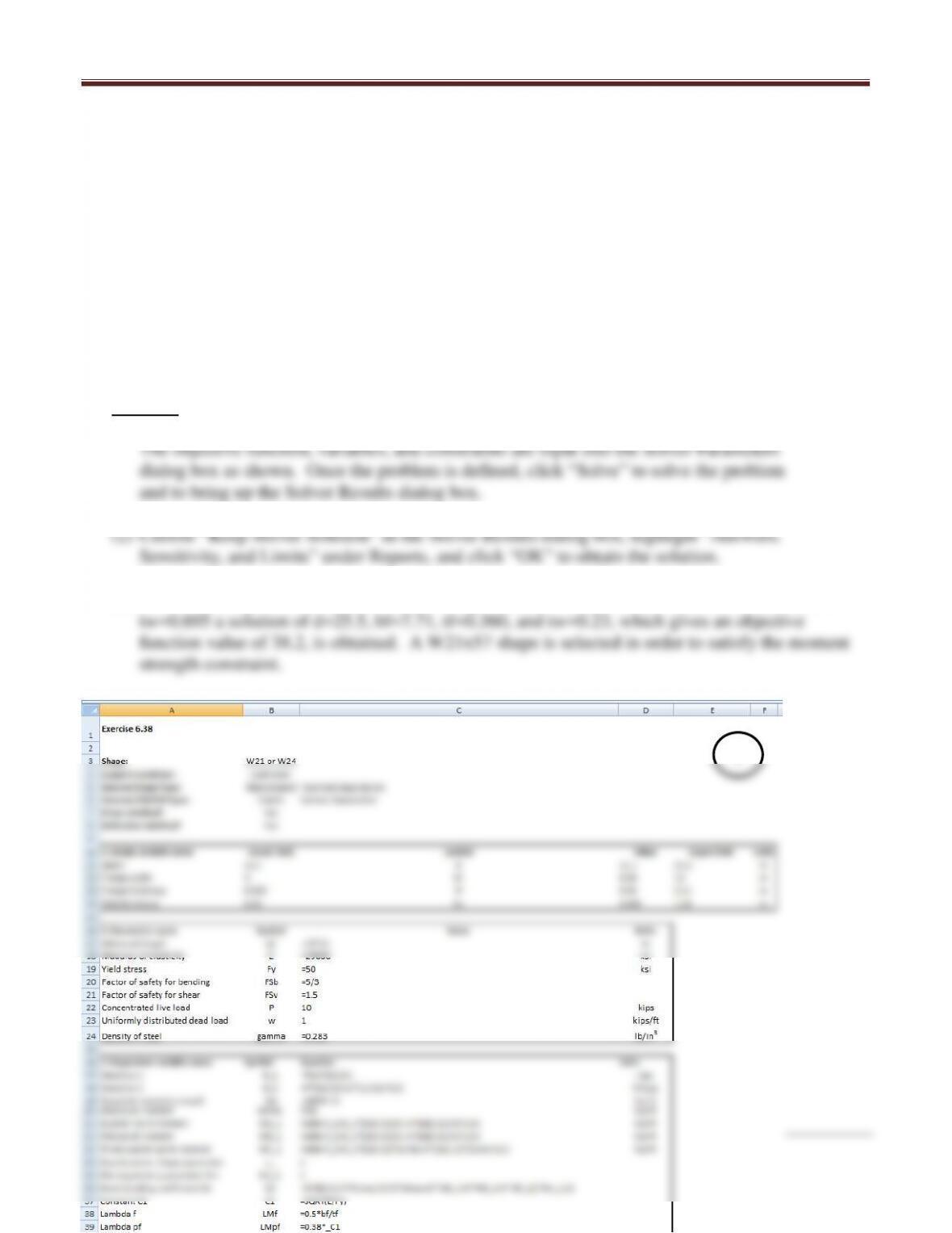
(1) One possible format for setting up the Excel worksheet for this problem is shown below.
1
Arora, Introduction to Optimum Design, 4e
14-50
14.46_______________________________________________________________________________
Continued.
3
2
1
Chapter 14 Practical Applications of Optimization
14.47_______________________________________________________________________________
Solve the following problem using the Excel Solver:
Design a cantilever beam of span 15 ft subjected to a dead load of 1 kips/ft and a point live load of
10 kips at the end. The material of the beam is A572 Grade 50 steel. Assume noncompact shape and
elastic LTB.
337.5 kip-ft, 37.5 kips
λ λ and λ λ
, 0.6 M
13.7 16.4, 5.0 16.0, 0.335 1.89, 0.23 1.18
aa
f pf w pw
pbr
n pa n
f fw
MV
LLL
M MM
db t t
= =
≤≤
<≤
≤≤
≤≤ ≤ ≤ ≤ ≤ ≤ ≤
Solution
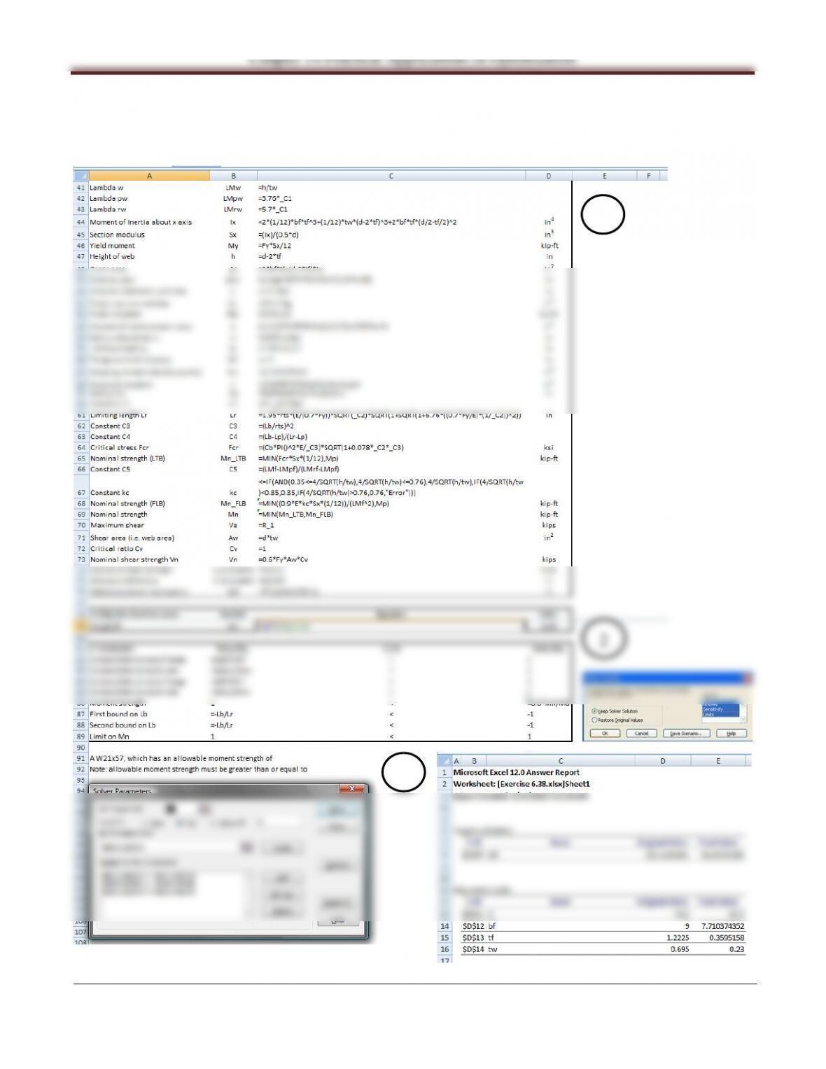
(1) One possible format for setting up the Excel worksheet for this problem is shown below.
(3) The answer report shows that for initial design variable values of d=19.6, bf=9, tf=1.223, and
1
Arora, Introduction to Optimum Design, 4e
14-52
14.47_______________________________________________________________________________
Continued.
3
2
1
Chapter 14 Practical Applications of Optimization
Section 14.11 Optimum Design of Telecommunication Poles
14.48_______________________________________________________________________________
Solve the following problem using the Excel Solver:
Solve the problem of Example 14.10 for a pole of height 40 m.
Solution
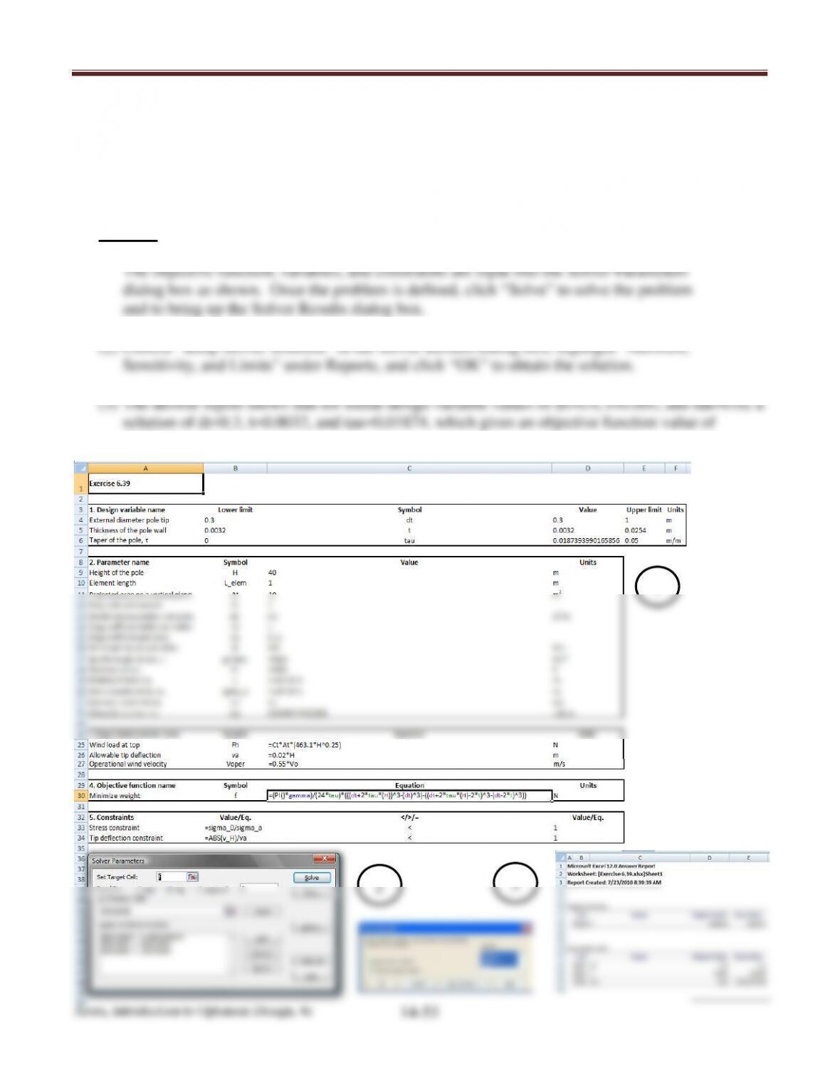
(1) One possible format for setting up the Excel worksheet for this problem is shown below.
33030.7, is obtained.
(4)
3
2
1

Arora, Introduction to Optimum Design, 4e
14-54
14.48_______________________________________________________________________________
Continued.
1
1
Chapter 14 Practical Applications of Optimization
14.49_______________________________________________________________________________
Solve the following problem using the Excel Solver:
Solve the problem of Example 14.11 for a pole of height 40 m.
Solution
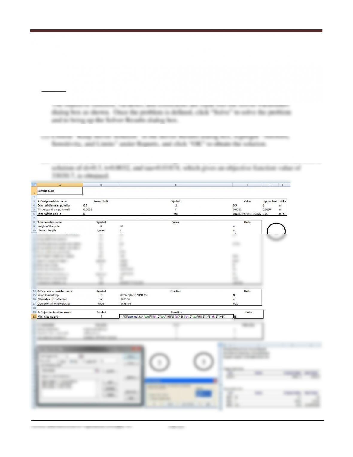
(1) One possible format for setting up the Excel worksheet for this problem is shown below.
(3) The answer report shows that for initial design variable values of dt=0.4, t=0.005, and tau=0.02 a

Arora, Introduction to Optimum Design, 4e
14-56
14.49_______________________________________________________________________________
Continued.
1
1
Chapter 14 Practical Applications of Optimization
14.50_______________________________________________________________________________
Solve the following problem using the Excel Solver:
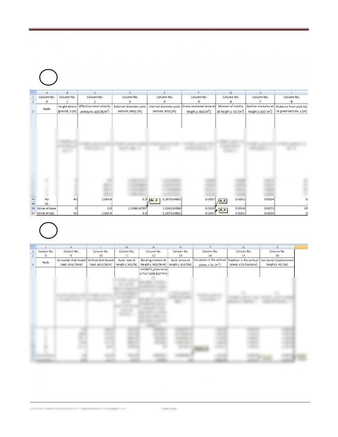
Solve the problem of Example 14.12 for a pole of height 40m.
Solution
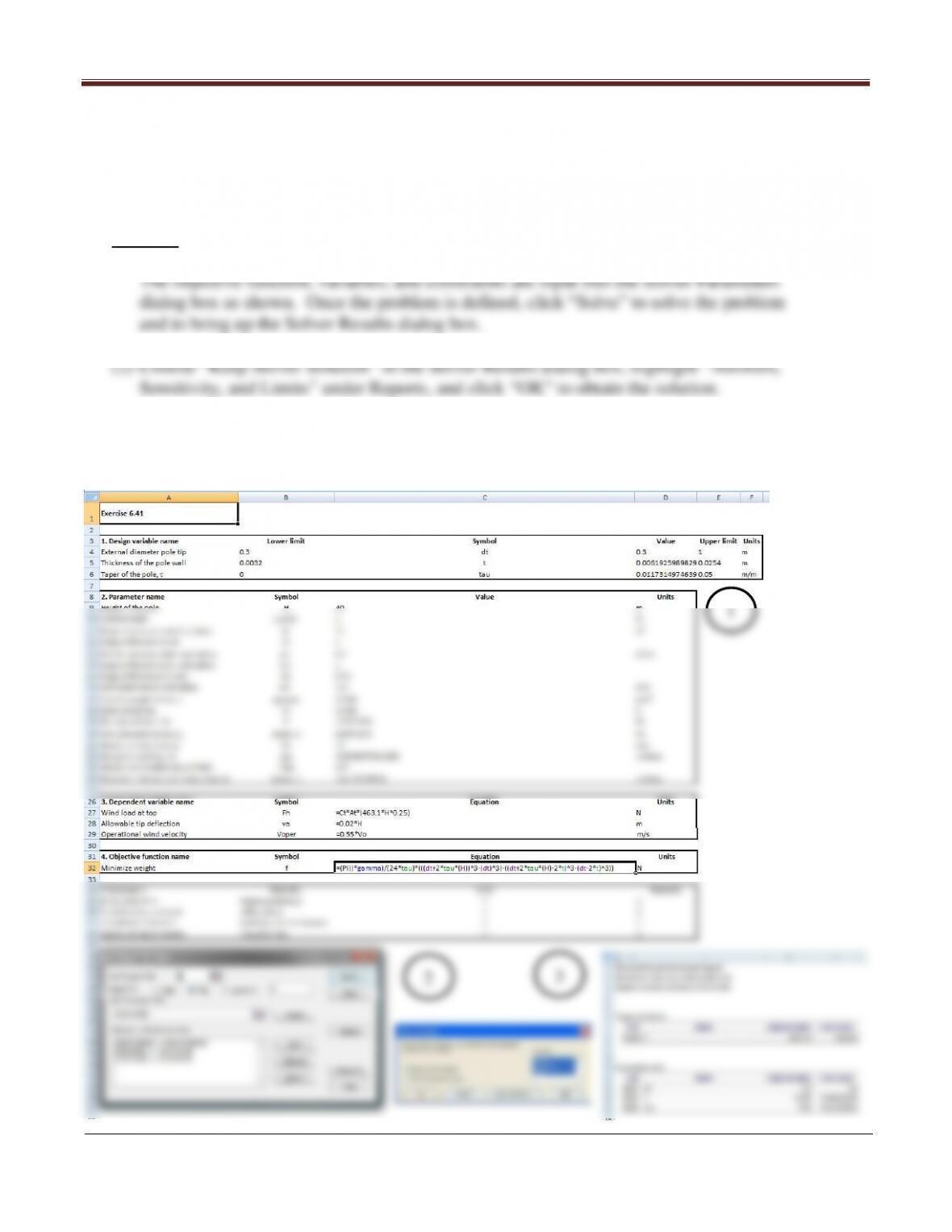
(1) One possible format for setting up the Excel worksheet for this problem is shown below.
(3) The answer report shows that for initial design variable values of dt=0.4, t=0.005, and tau=0.02 a
solution of dt=0.3, t=0.00619, and tau=0.01173, which gives an objective function value of
46614, is obtained.
1
3
Chapter 14 Practical Applications of Optimization
14.50_______________________________________________________________________________
Continued.
1
1