Chapter 13 More on Numerical Methods for Constrained Optimum Design
13.17 _______________________________________________________________________________
Refer to Exercise 12.6 for detailed formulation
Iteration 1: Refer to Exercise 13.4.
Iteration 2:
2. Computed cost and constraint functions and their gradients are given in 11:4 as:
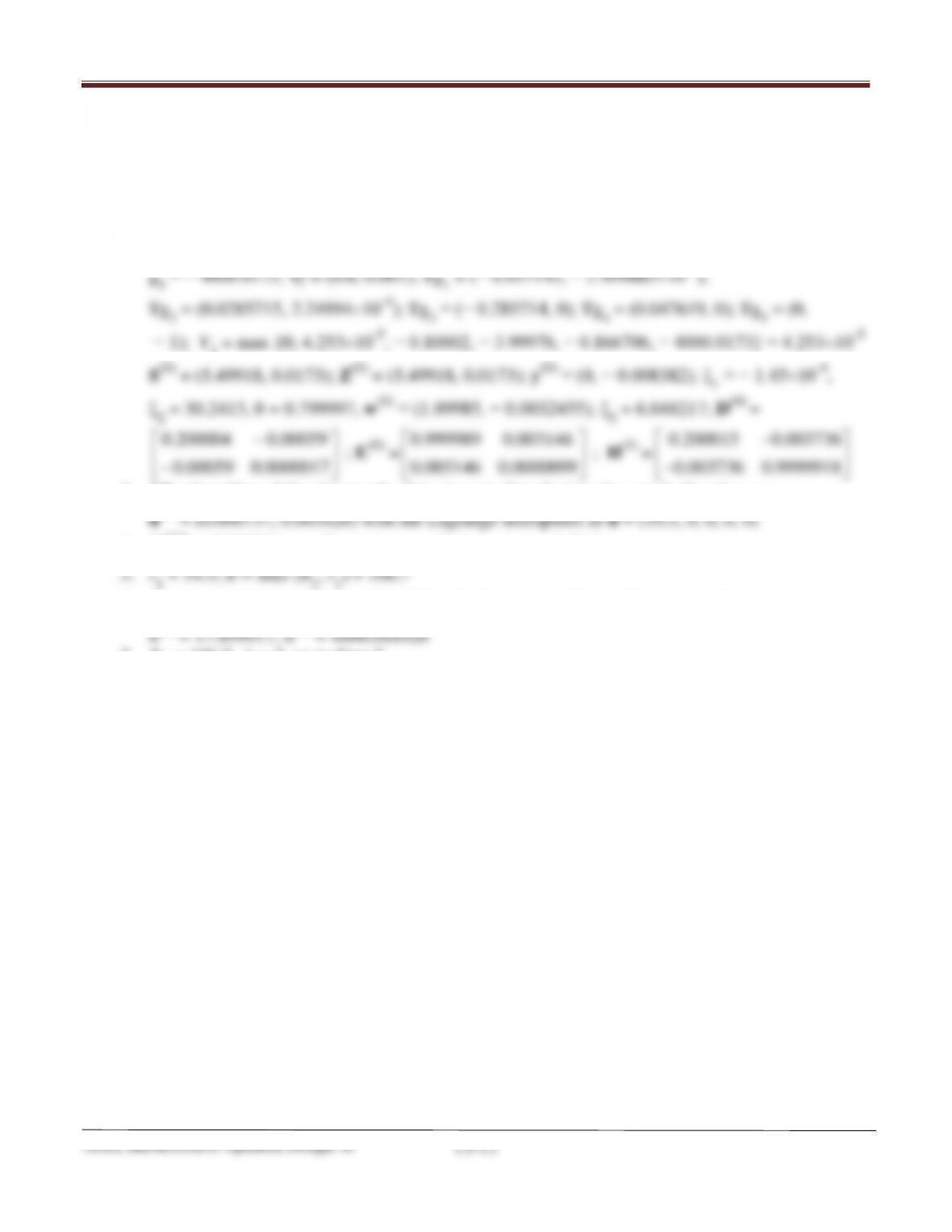
fo = 14.4995, g1 = 4.253×10⁻⁵, g2 = − 0.10002, g3 = − 3.99976, g4 = − 0.166706,
0.00059 0.0000017
−
0.003146 0.0000099
0.003736 0.9999918
−
3. QP subproblem defined using the data given in Step 2 gives the search direction as
4. ||d(1)|| = 0.00179 >
ε
2; Convergence criteria are not satisfied.
6. Step size at the 1st trial (to = 1) satisfies the descent condition. Design is updated as
7. R2 = 106.7, k = 2, go to Step 2.
Arora, Introduction to Optimum Design, 4e
13-14
13.18 _______________________________________________________________________________
Refer to Exercise 12.7 for detailed formulation
Iteration 1: Refer to Exercise 13.5
Iteration 2:
2. Computed cost and constraint functions and their gradients are given in 13.5 as:
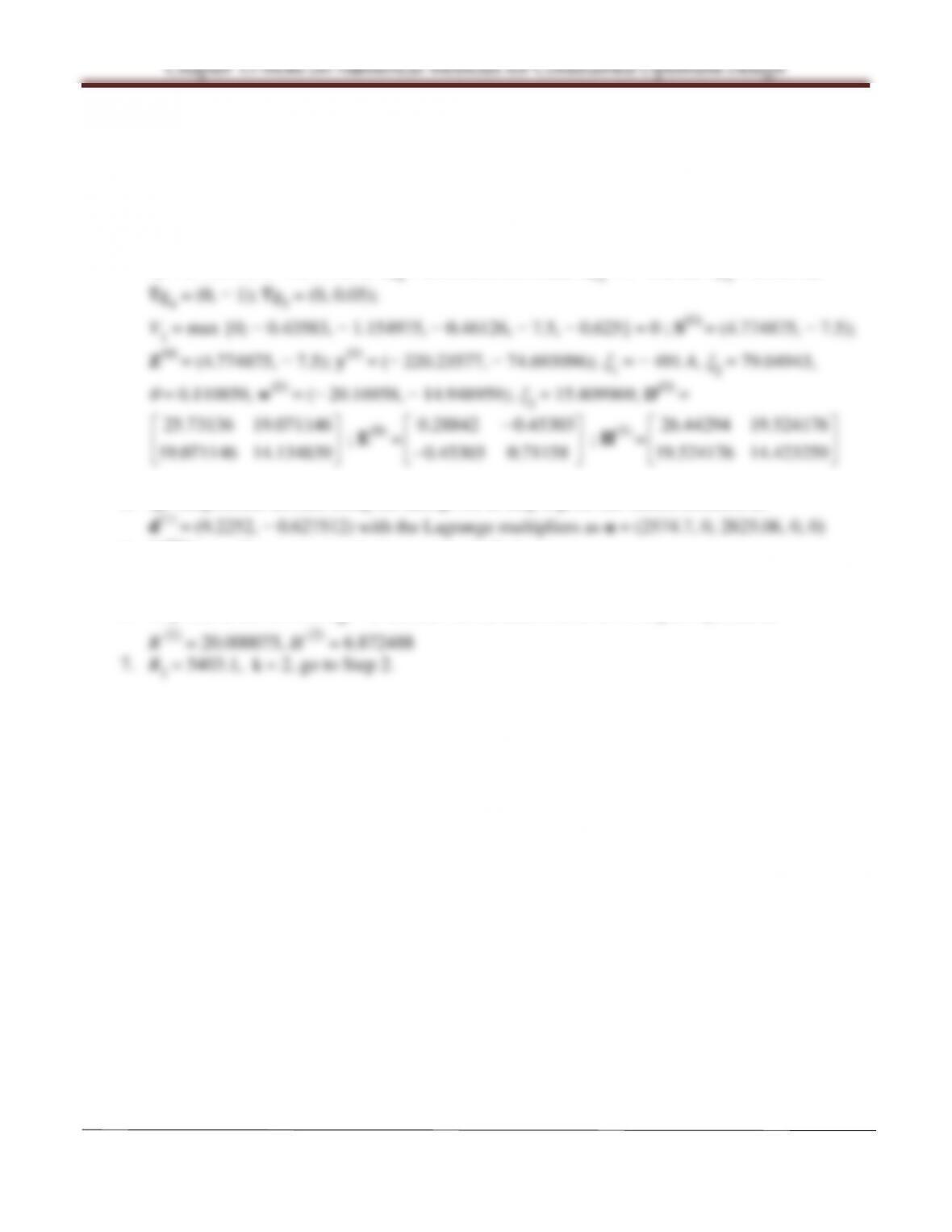
fo = − 2735.493, g1 = − 0.43583, g2 = −1.154975, g3 = − 0.46126, g4 = −7.5, g5 = − 0.625;
∇f = (− 507.754, − 364.7324); ∇g1 = (0.05236, 0.07522); ∇g2 = (− 0.2, 0); ∇g3 = (0.05, 0);
19.071146 14.134839
0.45303 0.71158
−
19.524176 14.423259
3. QP subproblem defined using the data given in Step 2 gives the search direction as
4. ||d(1)|| >
ε
2; Convergence criteria are not satisfied.
5. r1 = 5399.76; R = max (R1, r1) = 5403.1
6. Step size at the 1st trial (to = 1) satisfies the descent condition. Design is updated as
Chapter 13 More on Numerical Methods for Constrained Optimum Design
Arora, Introduction to Optimum Design, 4e
13-15
13.19 _______________________________________________________________________________
Refer to Exercise 12.8 for detailed formulation
Iteration 1: Refer to Exercise 13.6.
Iteration 2:
2. Computed cost and constraint functions and their gradients are given in 13.6 as:
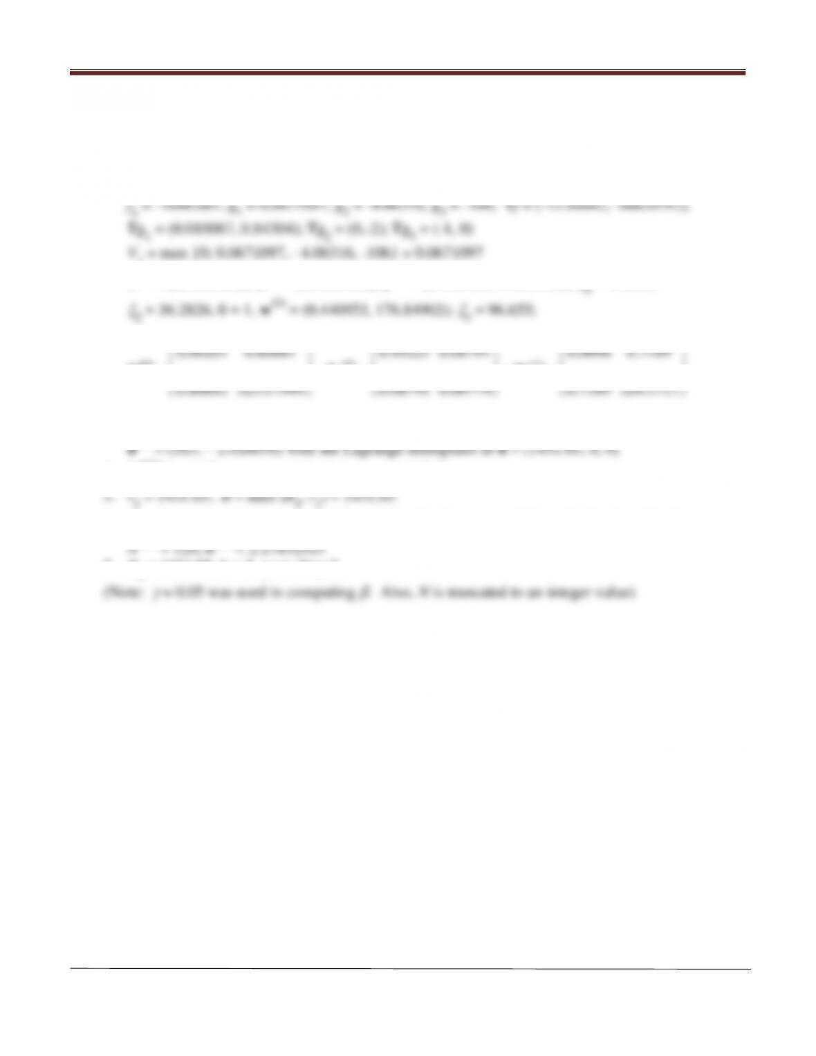
S(0) = (6, 0.53158); Z(0) = (6, 0.53158); y(0) = (0.440953, 176.84902);
ξ
3. QP subproblem defined using the data given in Step 2 gives the search direction as
4. ||d(1)|| >
ε
2; Convergence criteria are not satisfied.
6. Step size at the 4th trial (t4 = 0.125) satisfies the descent condition. Design is updated as
7. R2 = 1431.05, k = 2, go to Step 2.
Chapter 13 More on Numerical Methods for Constrained Optimum Design
13.20 _______________________________________________________________________________
Refer to Exercise 12.9 for detailed formulation
Iteration 1: Refer to Exercise 13.7.
Iteration 2:
2. Computed cost and constraint functions and their gradients are given in 13.7 as:
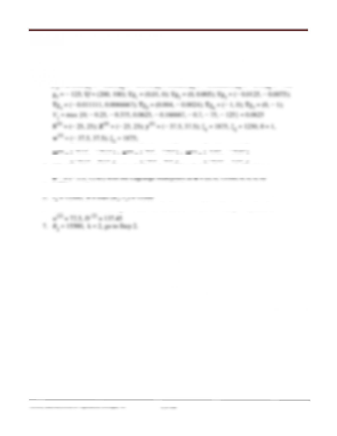
f o = 27500, g1 = − 0.25, g2 = − 0.375, g3 = 0.0625, g4 = − 0.166667, g5 = − 0.7, g6 = − 75,
D(0) =
0.75 0.75
0.75 0.75
−
−
; E(0) =
0.5 0.5
0.5 0.5
−
−
; H(1) =
1.25 0.25
0.25 1.25
−
−
3. QP subproblem defined using the data given in Step 2 gives the search direction as
4. ||d(1)|| >
ε
2; Convergence criteria are not satisfied.
6. Step size at the 1st trial (to = 1) satisfies the descent condition. Design is updated as
Arora, Introduction to Optimum Design, 4e
13-17
13.21 ______________________________________________________________________________
Refer to Exercise 12.10 for detailed formulation
Iteration 1: Refer to Exercise 13.8.
Iteration 2:
2. Computed cost and constraint functions and their gradients are given in 13.8 as:
fo = 395.383, h1 = 0.33729, g1 = 0.056233, g2 = − 0.37082, g3 = − 0.51548, g4 = − 9.69034,
4.445505 1.07918
−
0.13473 0.9815
4.580235 1.09768
−
d(1)= (− 0.533584, − 0.429772) with the Lagrange multipliers as u = (− 191.22, 80.51, 0, 0, 0, 0)
5. r 1 = 271.73; R = max (R1, r1) = 271.73
6. Step size at the 1st trial (to = 1) satisfies the descent condition. Design is updated as
7. R2 = 271.73, k = 2, go to Step 2.
Chapter 13 More on Numerical Methods for Constrained Optimum Design
Arora, Introduction to Optimum Design, 4e
13-18
13.22_______________________________________________________________________________
Refer to Exercise 12.11 for detailed formulation
Iteration 1: Refer to Exercise 13.9.
Iteration 2:
2. Computed cost and constraint functions and their gradients are given in 13.9 as:
3. QP subproblem defined using the data given in Step 2 gives the search direction as
4. ||d(1)|| >
ε
2; Convergence criteria are not satisfied.
6. Step size at the 1st trial (to = 1) satisfies the descent condition. Design is updated as
Chapter 13 More on Numerical Methods for Constrained Optimum Design
Arora, Introduction to Optimum Design, 4e
13-19
13.23 _______________________________________________________________________________
Refer to Exercise 12.12 for detailed formulation
Iteration 1: Refer to Exercise 13.10.
Iteration 2:
2. Computed cost and constraint functions and their gradients are given in 13.10 as:
f o = 18578.5548, g1 = 0.170573, g2 = −1.875, g3 = − 4, g4 = −1.875;
y(0) = (− 232.07428, 249.67847, − 83.01308); ξ1 = 571.4473, ξ2 = 3.03125, ξ3 = 571.4473,
D(0) =
94.24924 101.39859 33.713
109.09027 36.27032
. 12.05916symm
−
−
; E(0) =
0.12887 0.30928 0.12887
0.74227 0.30928
. 0.12887symm
−
−
;
H(1) =
95.12037 101.08931 33.58413
109.348 35.96104
. 12.93029symm
−
−
3. QP subproblem defined using the data given in Step 2 gives the search direction as
5. r1 = 14460.78; R = max (R1, r1) = 14460.78
Chapter 13 More on Numerical Methods for Constrained Optimum Design
Arora, Introduction to Optimum Design, 4e
13-20
13.24 ______________________________________________________________________________
Refer to Exercise 12.13 for detailed formulation
Iteration 1: Refer to Exercise 13.11.
Iteration 2:
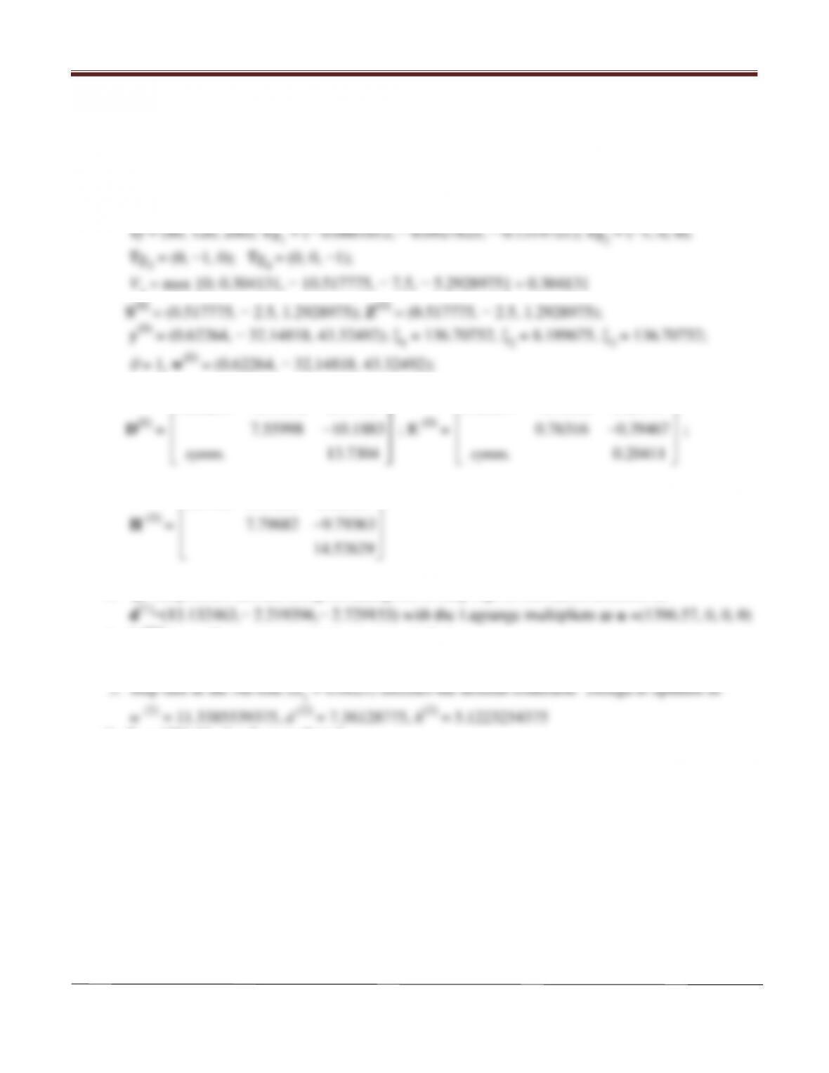
2. Computed cost and constraint functions and their gradients are given in 13.11 as:
S (0)= (1.492135, − 4); Z (0)= (1.492135, − 4); y(0)= (1576.5709, −1462.6373);
ξ
D(0)=
303.00793 281.11054
281.11054 260.79561
−
−
;E (0)=
0.12216 0.32746
0.32746 0.87784
−
−
;
303.88577 280.78308
−
d(1) = (− 0.199715, 2.621956) with the Lagrange multipliers as u = (− 48385.51, 0, 0, 0)
4. ||d(1)|| >
ε
6. Step size at the 1st trial (
α
Chapter 13 More on Numerical Methods for Constrained Optimum Design
Arora, Introduction to Optimum Design, 4e
13-21
13.25 ______________________________________________________________________________
Refer to Exercise 12.14 for detailed formulation
Iteration 1: Refer to Exercise 13.12.
Iteration 2:
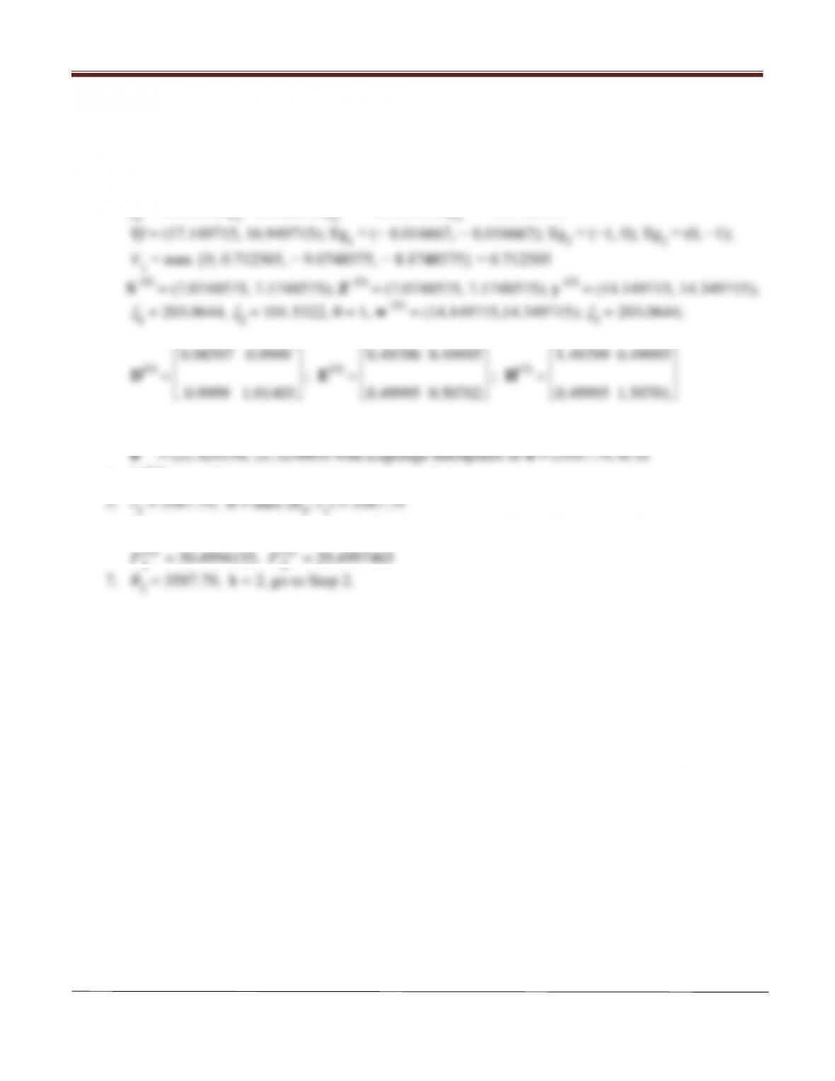
2. Computed cost and constraint functions and their gradients are given in 13.12 as:
fo = 2800.0015, g1 = 0.304131, g2 = −10.517775, g3 = − 7.5, g4 = − 5.2928975;
0.00284 0.14642 0.19733
. 13.7304symm
−
0.03274 0.15806 0.08174
. 0.20411symm
−
0.9701 0.01164 0.11559
14.52629
3. QP subproblem defined using the data given in Step 2 gives the search direction as
4. ||d(1)|| > ε2; Convergence criteria are not satisfied.
5. r1 = 1396.57; R = max (R1, r1) = 1396.57
7. R2 = 1396.57, k = 2, go to Step 2.
Chapter 13 More on Numerical Methods for Constrained Optimum Design
Arora, Introduction to Optimum Design, 4e
13-22
13.26 _______________________________________________________________________________
Refer to Exercise 12.15 for detailed formulation
Iteration 1: Refer to Exercise 13.13.
Iteration 2:
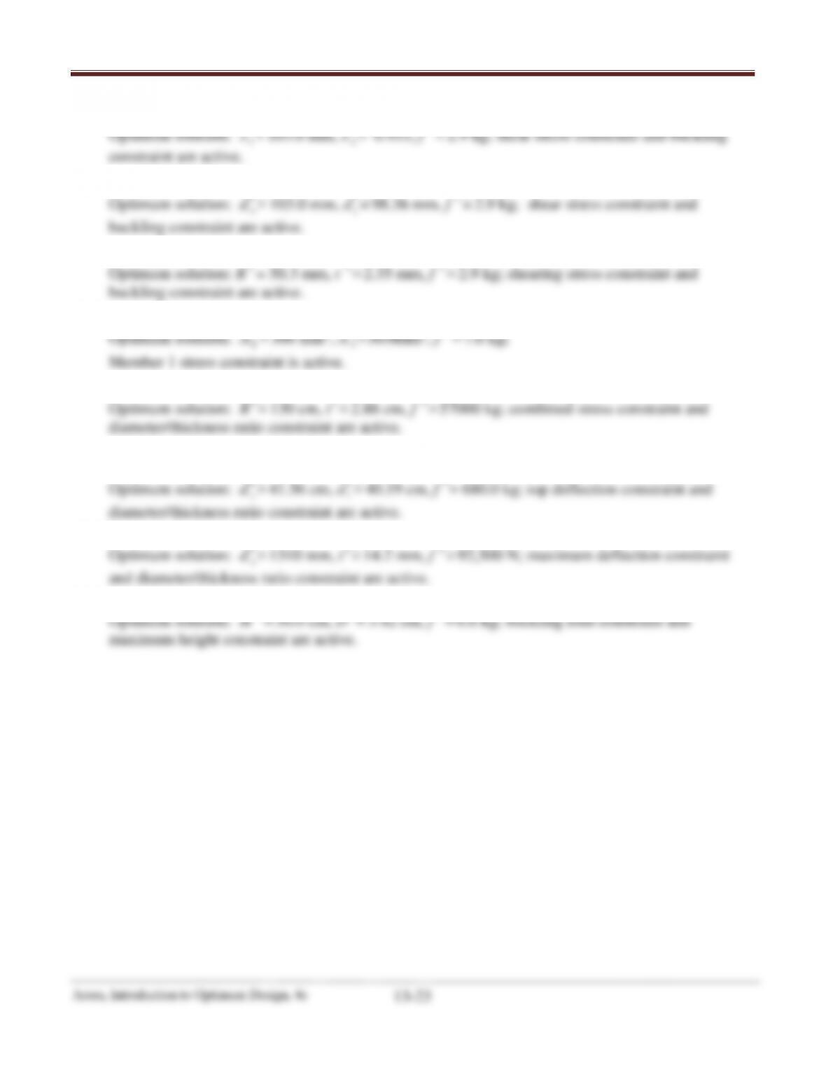
2. Computed cost and constraint functions and their gradients are given in 13.13 as:
fo = 147.0114, g1= 0.712505, g2 = − 9.0748575, g3 = − 8.1748575;
0.98597 0.9999
0.9999 1.01403
0.49298 0.49995
0.49995 0.50702
1.49299 0.49995
0.49995 1.50701
3. QP subproblem defined using the data given in Step 2 gives the search direction as
4. ||d(1)|| >
ε
2; Convergence criteria are not satisfied.
6. Step size at the 1st trial (t 0 = 1) satisfies the descent condition. Design is updated as
P
(2)
1
= 30.4994155, P
(2)
2
= 29.4997465
Chapter 13 More on Numerical Methods for Constrained Optimum Design
∗
∗
13.27 _______________________________________________________________________________
∗
∗
∗