Chapter 12 Numerical Methods for Constrained Optimum Design
Arora, Introduction to Optimum Design, 4e
12-39
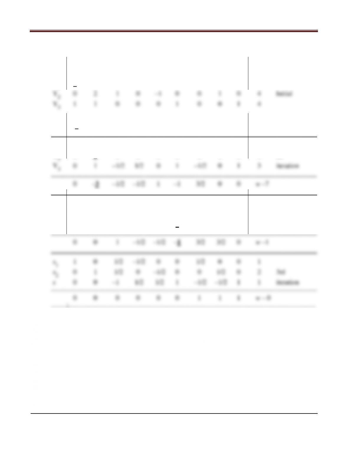
Table E12.33
______________________________________________________________________________
x1 x2 u ζ1 ζ2 s Y1 Y2 Y3 D
______________________________________________________________________________
Y1 2 0 1 –1 0 0 1 0 0 2
______________________________________________________________________________
–3 –3 –2 1 1 –1 0 0 0 w –10
______________________________________________________________________________
X 1 1 0 1/2 –1/2 0 0 1/2 0 0 1
Y2 0 2 1 0 –1 0 0 1 0 4 lst
______________________________________________________________________________
x1 1 0 1/2 –1/2 0 0 1/2 0 0 1
x2 0 1 1/2 0 –1/2 0 0 1/2 0 2 2nd
Y3 0 0 –1 1/2 1/2 1 –1/2 –1/2 1 1 iteration
——-|—-——-——————–————-——-—————-——-——-————-——-———
Chapter 12 Numerical Methods for Constrained Optimum Design
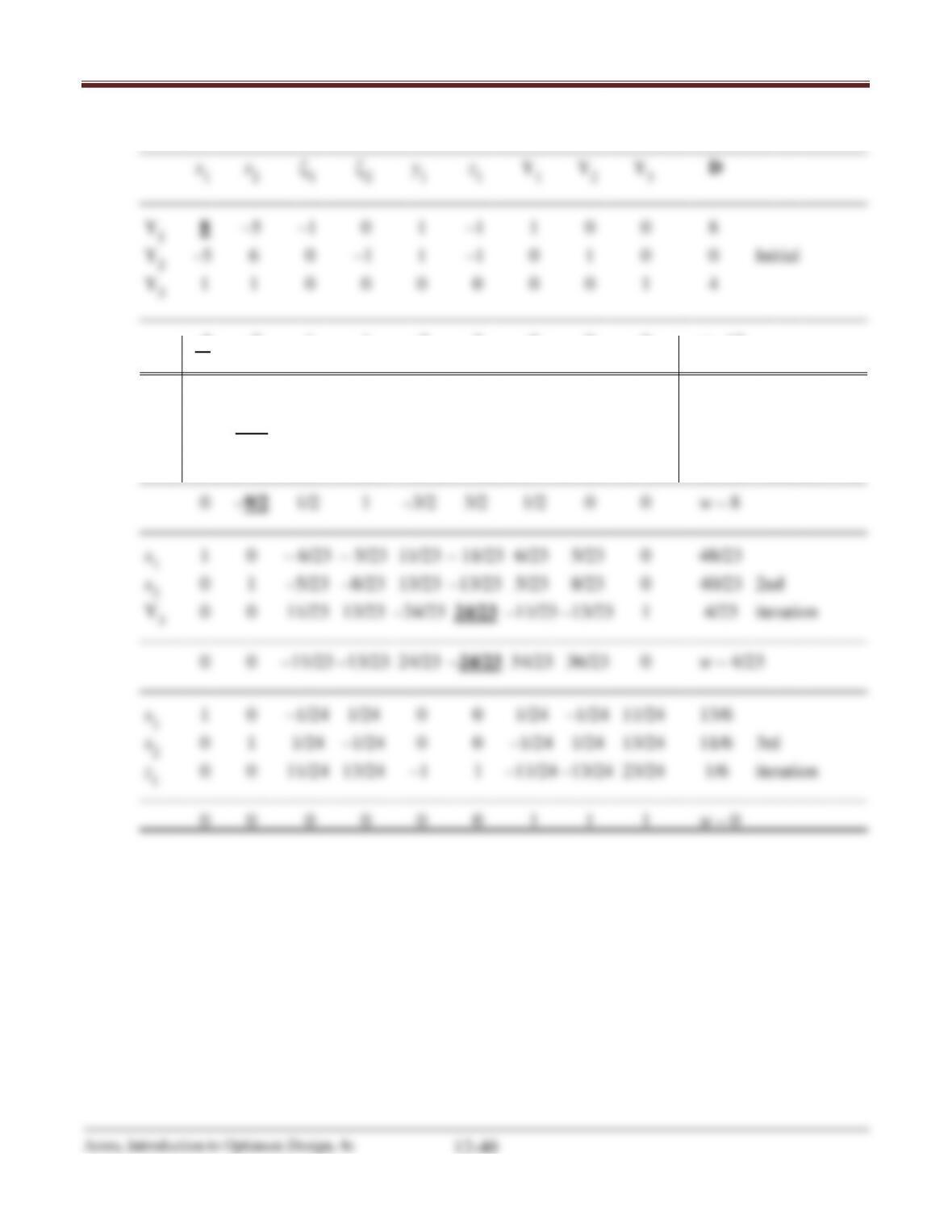
Table E12.34
-4 –2 1 1 –2 2 0 0 0 w –12
______________________________________________________________________________
x1 1 –5/8 –1/8 0 1/8 –1/8 1/8 0 0 1
Y2 0 23/8 –5/8 –1 13/8 –13/8 5/8 1 0 5 lst
Y3 0 13/8 1/8 0 –1/8 1/8 –1/8 0 1 3 iteration
Chapter 12 Numerical Methods for Constrained Optimum Design
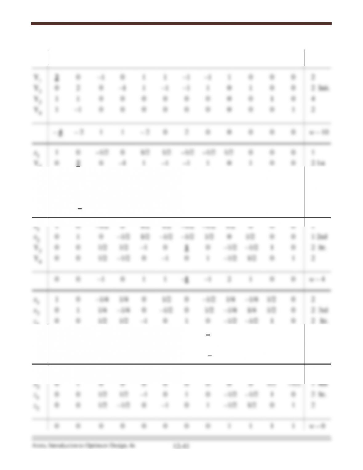
Table E12.35
____________________________________________________________________________________
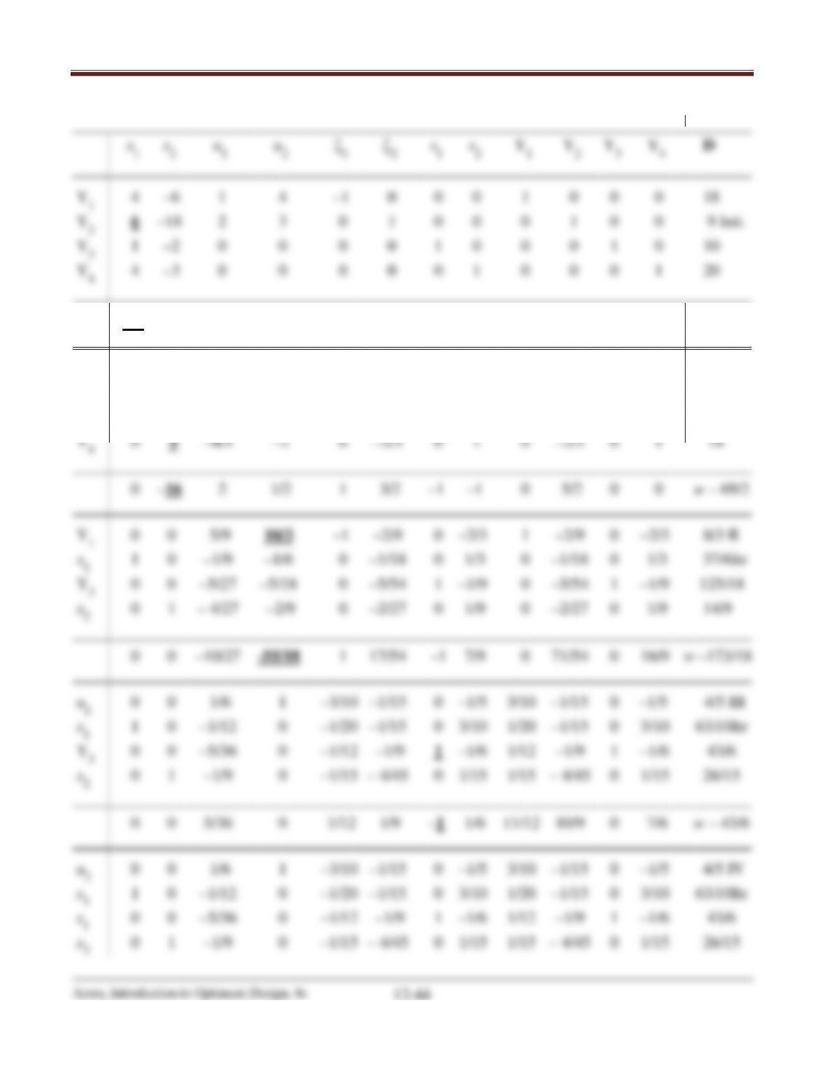
x1 x2 ζ1 ζ2 y1 y2 z1 z2 Y1 Y2 Y3 Y4 D
Y3 0 1 1/2 0 –1/2 –1/2 1/2 1/2 –1/2 0 1 0 3 Itr.
Y4 0 –1 1/2 0 –1/2 –1/2 1/2 1/2 –1/2 0 0 1 1
____________________________________________________________________________________
0 –2 –1 1 0 2 0 –2 2 0 0 0 w – 6
____________________________________________________________________________________
Y4 0 0 1/2 –1/2 0 –1 0 1 –1/2 1/2 0 1 2
____________________________________________________________________________________
0 0 –1/2 1/2 0 1 0 –1 3/2 1/2 1 0 w – 2
____________________________________________________________________________________
x1 1 0 0 0 0 0 0 0 0 0 1/2 1/2 3
Chapter 12 Numerical Methods for Constrained Optimum Design
Table E12.36
______________________________________________________________________________
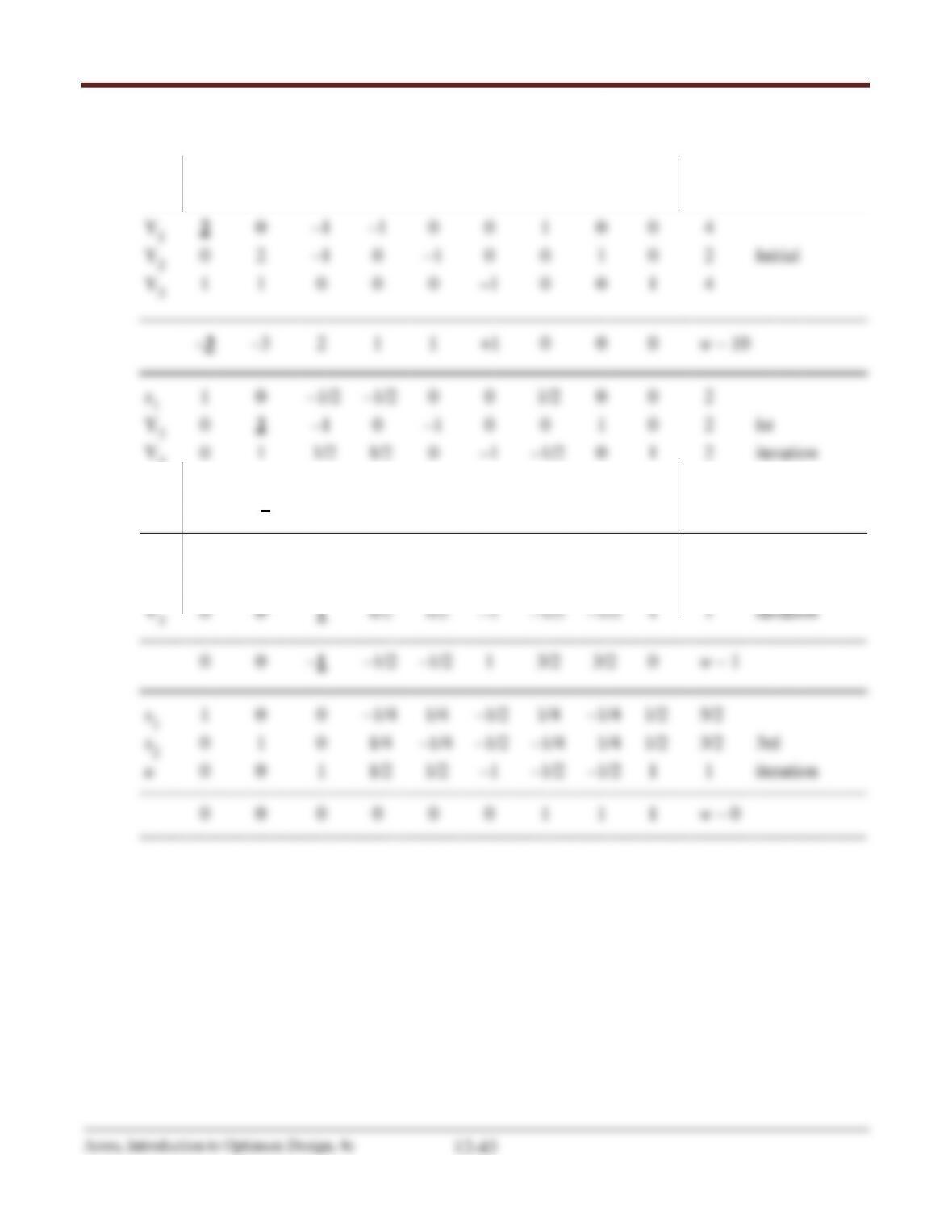
x1 x2 u ζ1 ζ2 s Y1 Y2 Y3 D
———–——-——————–————-——-—————-——-——-————-——-———
0 – 9/2 –3/2 1/2 1 –1 1/2 0 0 w – 8
______________________________________________________________________________
x1 1 0 11/23 –6/23 –5/23 0 6/23 5/23 0 48/23
x2 0 1 13/23 –5/23 –8/23 0 5/23 8/23 0 40/23 2nd
Chapter 12 Numerical Methods for Constrained Optimum Design
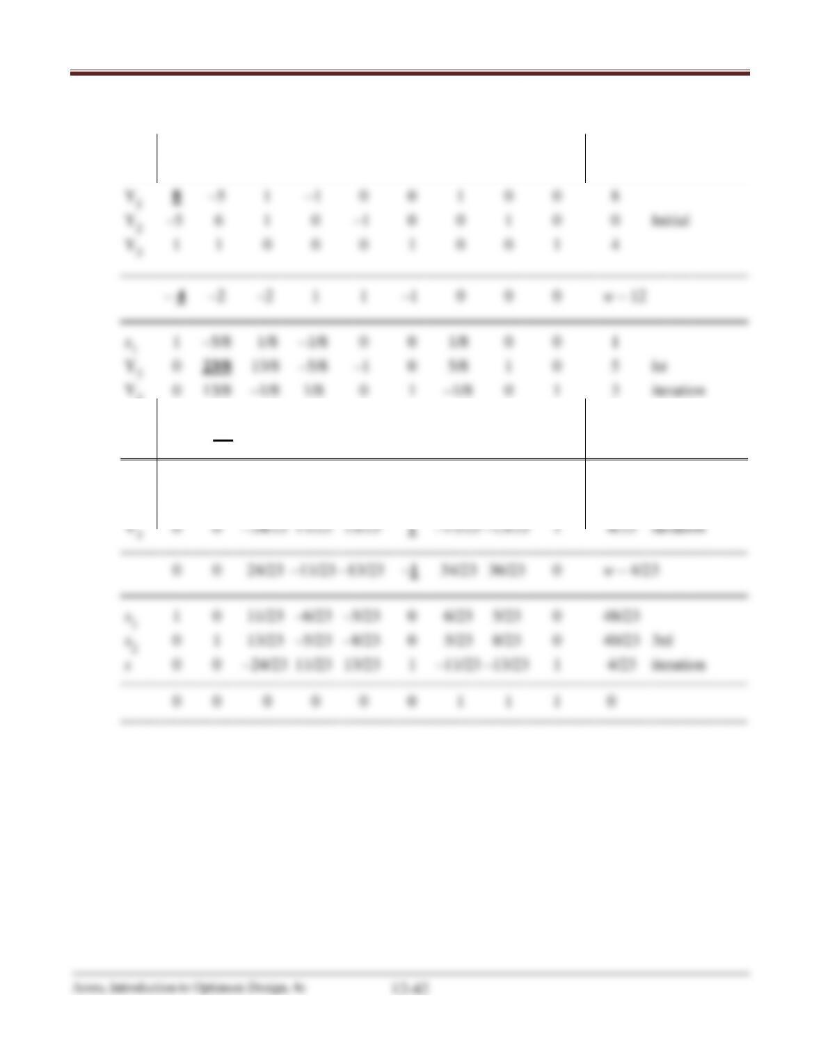
Table E12.37
______________________________________________________________________________
x1 x2 u ζ1 ζ2 s Y1 Y2 Y3 D
———–——-——————–————-——-—————-——-——-————-——-———
0 –3 1/2 –1/2 1 1 3/2 0 0 w – 4
______________________________________________________________________________
x1 1 0 –1/2 –1/2 0 0 1/2 0 0 2
x2 0 1 –1/2 0 –1/2 0 0 1/2 0 1 2nd
Chapter 12 Numerical Methods for Constrained Optimum Design
Table E12.38
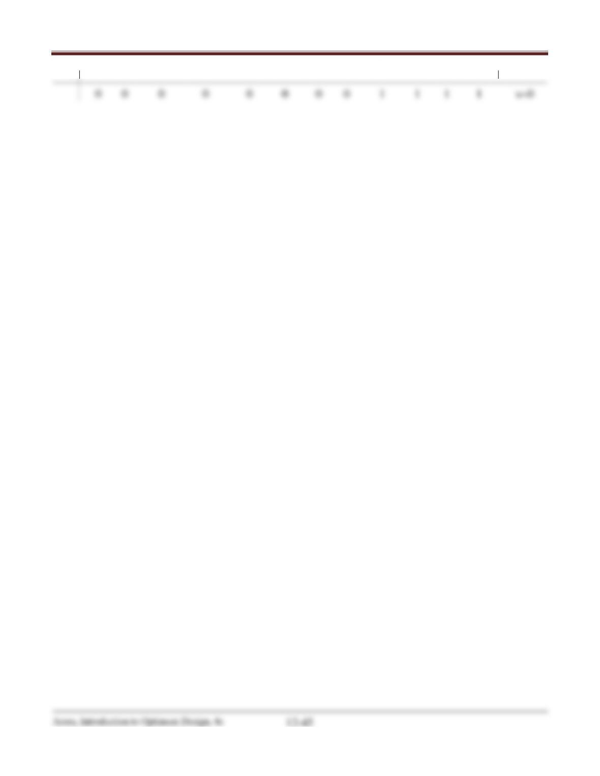
-15 29 –3 –7 1 –1 –1 –1 0 0 0 0 w – 57
____________________________________________________________________________________
Y1 0 6 –1/3 2 –1 –2/3 0 0 1 –2/3 0 0 12 I
x1 1 –3 1/3 1/2 0 1/6 0 0 0 1/6 0 0 3/2 Itr
Y3 0 1 –1/3 –1/2 0 –1/6 1 0 0 –1/6 1 0 17/2
Chapter 12 Numerical Methods for Constrained Optimum Design
____________________________________________________________________________________
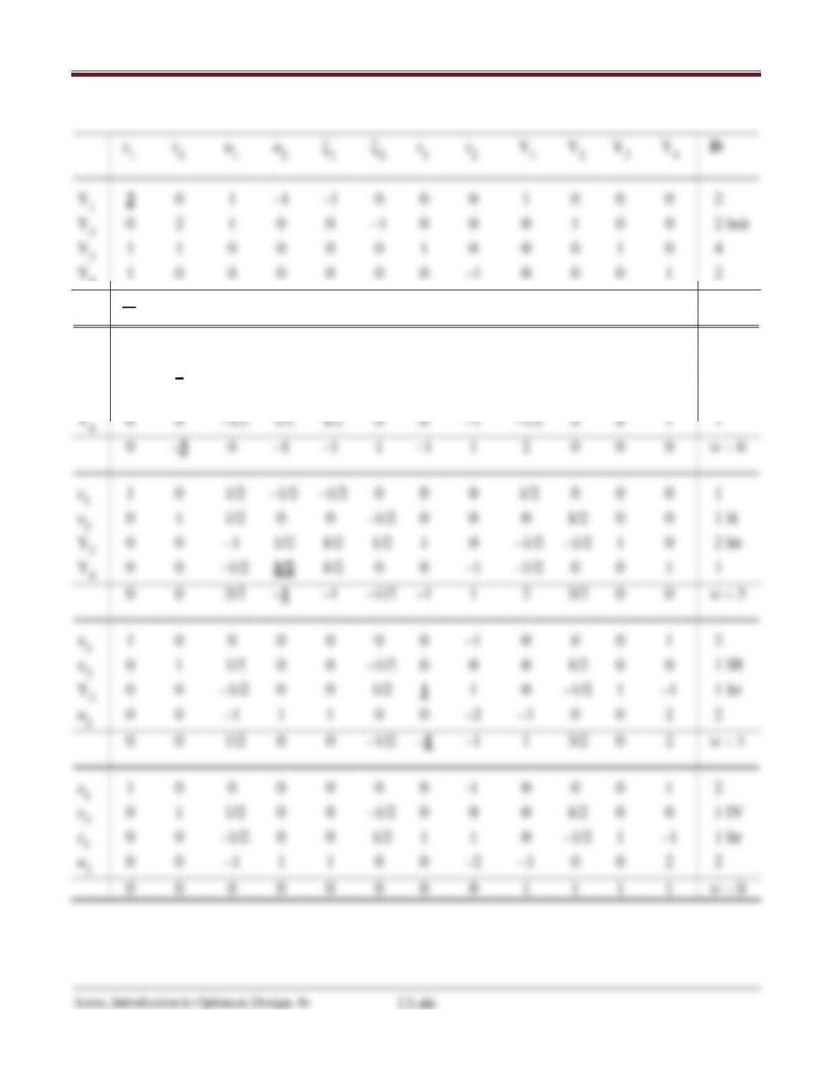
0 0 0 0 0 0 0 0 1 1 1 1 w-0
Chapter 12 Numerical Methods for Constrained Optimum Design
Table E12.39
-4 –3 –2 1 1 1 –1 1 0 0 0 0 w –10
____________________________________________________________________________________
x1 1 0 1/2 –1/2 –1/2 0 0 0 1/2 0 0 0 1
Y2 0 2 1 0 0 –1 0 0 0 1 0 0 2 I
Y3 0 1 –1/2 1/2 1/2 0 1 0 –1/2 0 1 0 3 Itr
Chapter 12 Numerical Methods for Constrained Optimum Design
12.41 _______________________________________________________________________________
Referring to Exercises 12.3 and 12.16, the QP subproblem at the point (250, 300) is defined as:
– 0.1d1 ≤ 24; 0.001d1 ≤ 0.75
12.42 _______________________________________________________________________________
Referring to Exercises 12.4 and 12.17, the QP subproblem at the point (12, 4) is defined as:
– 22.50374d1 – 22.50374d2 ≤ 89.01498
12.43 _______________________________________________________________________________
Referring to Exercises 12.5 and 12.18, the QP subproblem at the point (150, 150) is defined as:
12.44 _______________________________________________________________________________
Exercise 2.1 at the point h = 12m, A = 4000m2.
Exercise 2.1
A 100 × 100m lot is available to construct a multistory office building. At least 20,000m2 total floor
space is needed. According to a zoning ordinance, the maximum height of the building can be only
3.5, m2
Step 3: Definition of Design Variables
A = cross-sectional area of the building for each floor, m2
hA/3.5
≥
20,000, m2 (2)
Explicit Design Variable Constraints:
h
≥
3.5, m (4)
≤
≥
Substituting the given values the problem is formulated in the standard and normalized form as:
( , ) (0.6 0.001 )f hA h A= +
5
−
2
Arora, Introduction to Optimum Design, 4e
12-49
31 3.5 0gh=−≤
421 1 0gh= −≤
A
2[7.14286 10 ,0.0001 7.14286 10 ] [0.02857,1.857 10 ]gA h
Referring to Exercises 12.6 and 12.19, the QP subproblem at the point (12, 4000) is defined as:
f
= 0.6d1 + 0.001d2 + 0.5(d2
1 + d2
2);
subject to ̅1=– 0.057143d1 – 0.00017143d2 + 0.3143 ≤ 0
Chapter 12 Numerical Methods for Constrained Optimum Design
12.45 _______________________________________________________________________________
Referring to Exercises 12.7 and 12.20, the QP subproblem at the point (6, 15) is defined as:
12.46 _______________________________________________________________________________
Referring to Exercises 12.8 and 12.21, the QP subproblem at the point (100, 2) is defined as:
f
12.47 _______________________________________________________________________________
Referring to Exercises 12.9 and 12.22, the QP subproblem at the point (100, 100) is defined as:
0.005d1 – 0.005d2 ≤ 0.5
12.48 _______________________________________________________________________________
Referring to Exercises 12.10 and 12.23, the QP subproblem at the point (6, 16) is defined as:
f
= 138.2301d1 + 37.699d2 + 0.5(d2
1 + d2
2);
subject to 1.0053d1 + 0.1885d2 = – 2.01593
Arora, Introduction to Optimum Design, 4e
12-51
12.49 _______________________________________________________________________________
Referring to Exercises 12.11 and 12.24, the QP subproblem at the point (5, 10) is defined as:
12.50 _______________________________________________________________________________
Referring to Exercises 12.12 and 12.25, the QP subproblem at the point (5, 5, 5) is defined as:
12.51 _______________________________________________________________________________
Referring to Exercises 12.13 and 12.26, the QP subproblem at the point (4, 8) is defined as:
12.52 _______________________________________________________________________________
Referring to Exercises 12.14 and 12.27, the QP subproblem at the point (10, 10, 4) is defined as:
12.53 _______________________________________________________________________________
Referring to Exercises 12.15 and 12.28, the QP subproblem at the point (2, 1) is defined as:
Chapter 12 Numerical Methods for Constrained Optimum Design
Arora, Introduction to Optimum Design, 4e
12-52
Section 12.7 The Constrained Steepest-descent Method
12.54 _______________________________________________________________________________
2. The constrained steepest-descent method solves two subproblems: the search direction and
step size determination. True
4. The QP subproblem in the CSD method is strictly convex. True
6. Constraint violations play no role in step size determination in the CSD method. False
8. Constraints must be evaluated during line search in the CSD method. True
12.55 _______________________________________________________________________________
For the following problem, calculate the descent function values Φ0, Φ1, and Φ2 at the trial step
12.56 _______________________________________________________________________________
12.57 _______________________________________________________________________________
Chapter 12 Numerical Methods for Constrained Optimum Design
Arora, Introduction to Optimum Design, 4e
12-53
12.58 _______________________________________________________________________________
Refer to Exercise 12.6 for detailed formulation; Step size
1.0
QP Subproblem:
Minimize
= 0.61+ 0.0012+1
2�12+22�
Subject to
̅1=−0.0571−0.00017142+ 0.3143 ≤0
̅1 is active at the optimum solution given as
d = (5.514, 0.0174), u* = (107.269, 0, 0, 0, 0, 0), ̅P
* = 18.51.
Descent Function Values:
Initial values at x(0) include
The necessary condition must be checked in which r0 is calculated, giving
=1
The necessary condition is then met if
R = max(R0, r0) = max(1, 107.269) = 107.269
Then we re-calculate the cost function and constraints at the new given point
Chapter 12 Numerical Methods for Constrained Optimum Design
f = 0.6(12.5514) + 0.001(4000.00174) = 11.53
g5 = 12.5514/21 – 1 = –0.4023 ≤ 0 (Inactive)
The maximum constraint violation is then calculated
The new descent function is then calculated as
The next trial point is then calculated
Then we re-calculate the function and constraints at the new given point
f = 0.6(13.444) + 0.001(4000.0046) = 12.066
Arora, Introduction to Optimum Design, 4e
12-55
12.59 _______________________________________________________________________________
Refer to Exercise 12.7 for detailed formulation; Step size
0.5
12.61 _______________________________________________________________________________
Refer to Exercise 12.9 for detailed formulation; Step size
0.5
12.62 _______________________________________________________________________________
12.63 ______________________________________________________________________________
Refer to Exercise 12.11 for detailed formulation; Step size
1.0
12.64 _______________________________________________________________________________
12.65 _______________________________________________________________________________
Refer to Exercise 12.13 for detailed formulation; Step size
0.5