Chapter 12 Numerical Methods for Constrained Optimum Design
Arora, Introduction to Optimum Design, 4e
12-1
CHAPTER
12
Numerical Methods for
Constrained Optimum Design
Section 12.1 Basic Concepts Related to Numerical Methods
12.1 ______________________________________________________________________________
Answer True or False.
1. The basic numerical iterative philosophy for solving constrained and unconstrained problems
2. Step size determination is a one-dimensional problem for unconstrained problems. True
4. An inequality constraint gi(x)≤0 is violated at x(k) if gi(x(k)) > 0. True
6. An equality constraint hi(x)=0 is violated at x(k) if hi(x(k)) < 0. True
8. In constrained optimization problems, search direction is found using the cost gradient only.
9. In constrained optimization problems, search direction is found using the constraint gradients
10. In constrained problems, the descent function is used to calculate the search direction. False
12. Cost function can be used as a descent function in unconstrained problems. True
14. A robust algorithm guarantees convergence. True
15. A feasible set must be closed and bounded to guarantee convergence of algorithms. True
Section 12.2 Linearization of the Constrained Problem
12.2 ________________________________________________________________________________
Answer True or False.
1. Linearization of cost and constraint functions is a basic step for solving nonlinear optimization
2. General constrained problems cannot be solved by solving a sequence of linear programming
3. In general, the linearized sub-problem without move limits may be unbounded. True
4. The sequential linear programming method for general constrained problems is guaranteed to
5. Move limits are essential in the sequential linear programming procedure. True
Chapter 12 Numerical Methods for Constrained Optimum Design
Arora, Introduction to Optimum Design, 4e
12-2
12.3 ________________________________________________________________________________
Formulate the following design problem, transcribe it into the standard form, create a linear
approximation at the given point, and plot the linearized sub-problem on a graph.
The beam design problem formulated in Section 3.8 at the point (b, d) = (250, 300) mm
Solution:
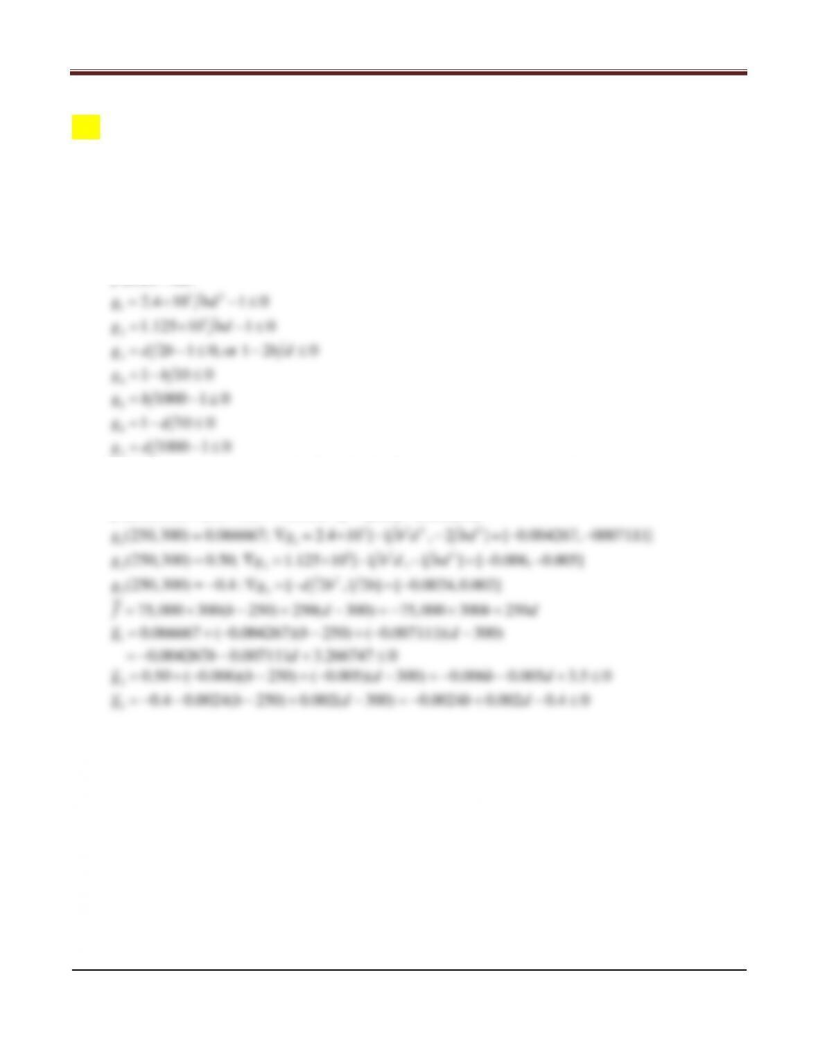
Writing the problem in the normalized form, we get:
(, ) ;f b d bd=
72
7
Only f, g1, g2 and g3 need to be linearized; other constraints are already linear.
b = 250 mm, d = 300 mm
(250,300) 250 300 75,000;f=×=
[ , ] [300, 250]f db∇= =
7 22 3
30.4 0.0024( 250) 0.002( 300) 0.0024 0.002 0.4 0g b d bd=−− − + − =− + − ≤
Chapter 12 Numerical Methods for Constrained Optimum Design
12.4 ________________________________________________________________________________
Formulate the following design problem, transcribe it into the standard form, create a linear
approximation at the given point, and plot the linearized sub-problem on a graph.
The tubular column design problem formulated in Section 2.7 at the point (R, t) = (12, 4) cm.
Let
50 ,P kN=
210 ,E GPa=
500 ,l cm=
250 ,
a
MPa
σ
=
and
3
7850 .
kg m
ρ
=
Solution:
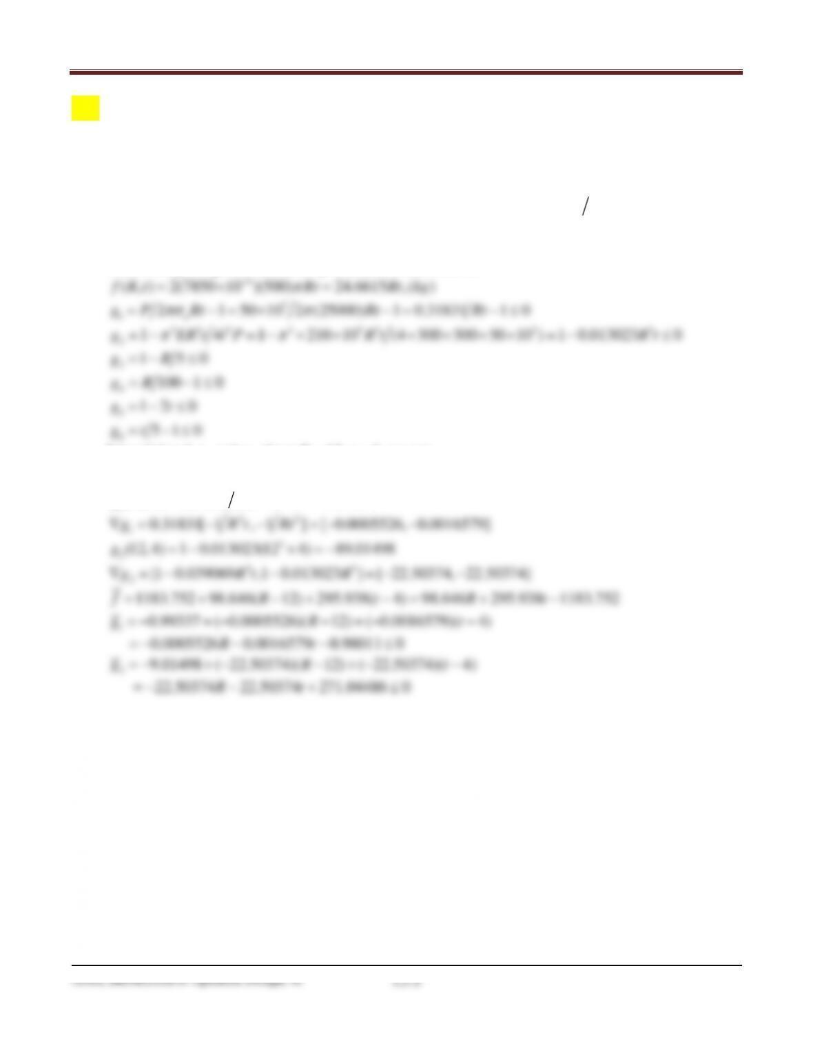
Substituting the given values the problem is formulated as:
6
−
6
Linearizing f, g1 and g2 about R = 12, t = 4, we get:
(12, 4) 24.6615 12 4 1183.752;f= × ×=
(12, 4) [24.6615 , 24.6615 ] [98.646, 295.938]f tR∇= =
1
(12, 4) 0.31831 (12 4) 1 0.99337g= × −=−
22
1
0.31831[ 1 , 1 ] [ 0.0005526, 0.0016579]g R t Rt∇= − − =− −
3
2(12, 4) 1 0.013023(12 4) 89.01498g=− ×=−
23
2
[1 0.039069 ,1 0.013023 ] [ 22.50374, 22.50374]g Rt R∇=− − =− −
1183.752 98.646( 12) 295.938( 4) 98.646 295.938 1183.752f R t Rt= + − + −= + −
10.99337 ( 0.0005526)( 12) ( 0.0016579)( 4)g Rt=− +− − +− −
0.0005526 0.0016579 0.98011 0Rt=− − −≤
2
9.01498 ( 22.50374)( 12) ( 22.50374)( 4)g Rt=− +− − +− −
22.50374 22.50374 271.04486 0Rt=− −+ ≤
Arora, Introduction to Optimum Design, 4e
12-4
12.5 ________________________________________________________________________________
Formulate the following design problem, transcribe it into the standard form, create a linear
approximation at the given point, and plot the linearized sub-problem on a graph.
The wall bracket problem formulated in Section 4.9.1 at the point (A1, A2) = (150, 150) cm2.
Solution:
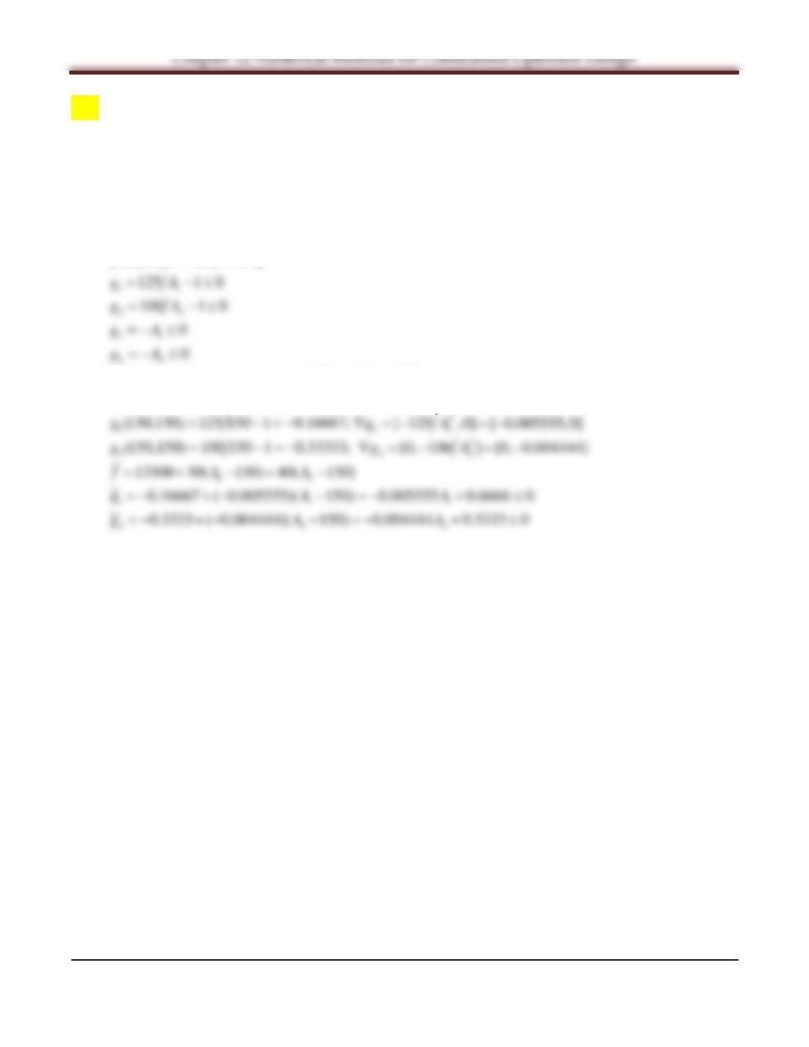
Substituting the given values the problem is formulated as:
12 1 2
(A , A ) 50 40f AA= +
42
Linearizing f, g1 and g2 at A1 = 150 and A2 = 150, we get:
(150,150) (50 150) (40 150) 13500;f=× +× =
(150,150) [50, 40]f∇=
2
2 22
Chapter 12 Numerical Methods for Constrained Optimum Design
12.6 ________________________________________________________________________________
Exercise 2.1 at the point h = 12 m, A = 4000 m2.
Solution:
Substituting the given values the problem is formulated as:
( , ) (0.6 0.001 )f hA h A= +
5
−
421 1 0gh= −≤
50gA=−≤
Linearizing f, g1 and g2 about h = 12, A = 4000, we get:
(12, 4000) (0.6 12) (0.001 4000) 11.2;f= ×+ × =
(12, 4000) [0.6,0.001]f∇=
5
−
4
10.3143 ( 0.057143)( 12) ( 1.7143 10 )( 4000)g hA
−
= +− − +− × −
4
−
44
2
0.25714 0.02857( 12) 1.857 10 ( 4000) 0.02857 1.857 10 1.34284 0g h A hA
−−
=− + −+× − = +× − ≤
Arora, Introduction to Optimum Design, 4e
12-6
12.7 ________________________________________________________________________________
Exercise 2.3 at the point (R, H) = (6, 15) cm.
Solution:
Substituting the given values the problem is formulated as:
2
(, )f RH RH
π
= −
520 1 0gH= −≤
Linearizing f and g1 about R = 6, H = 15, we get:
2
(6,15) 6 15 1696.46;f
π
=−× × =−
2
(12, 4) [ 2 , ] [ 565.487, 113.097]f RH R
ππ
∇ =− −=− −
Chapter 12 Numerical Methods for Constrained Optimum Design
12.8 ________________________________________________________________________________
Exercise 2.4 at the point R = 2 cm, N = 100.
Solution:
Substituting the given values the problem is formulated as:
( , ) 2 6.2832f N R lNR NR
π
=−=−
2 32
−
3
Linearizing f and g1 about R = 2, N = 100, we get:
(100, 2) 6.2832 100 2 1256.64;f=− × ×=−
(100, 2) [ 6.2832 , 6.2832 ] [ 12.5664, 628.32]f RN∇=− − =−−
32
1(100, 2) (1.5708 10 ) 100 2 1 0.3717g−
= × × × −=−
32 3 3
1
[1.5708 10 ,3.1416 10 ] [6.2832 10 , 0.62832]g R NR
−− −
∇= × × = ×
1256.64 ( 12.5664)( 100) ( 628.32)( 2) 12.5664 628.32 1256.64f N R NR=− +− − +− − =− − +
3
10.3717 (6.2832 10 )( 100) (0.62832)( 2)g NR
−
=− + × −+ −
3
6.2832 10 0.62832 2.25666 0NR
−
= ×+ − ≤
12.9 ________________________________________________________________________________
Exercise 2.5 at the point (W, D) = (100, 100) m.
Solution:
Substituting the given values the problem is formulated as:
( , ) 200 100fWD W D= +
1100 1 0gW= −≤
2200 1 0gD= −≤
Chapter 12 Numerical Methods for Constrained Optimum Design
12.10 ______________________________________________________________________________
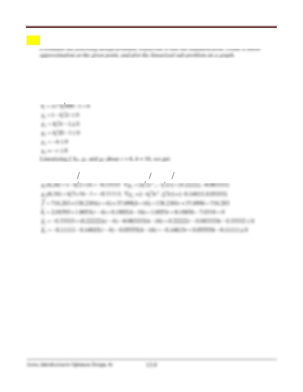
Exercise 2.9 at the point (r, h) = (6, 16) cm
Solution:
Substituting the given values the problem is formulated as:
2
(, ) 2f r h r rh
ππ
= +
2
2
(6,16) (6 ) 2 (6 16) 716.283;f
ππ
= + ×=
(6,16) [2 2 , 2 ] [138.2301, 37.699]f r hr
π ππ
∇=+ =
2
1
(6,16) 600 1 2.01593;h rh
π
= −=
2
1
[ 300, 600] [1.0053, 0.1885]h rh r
ππ
∇= =
2
12.11 _______________________________________________________________________________
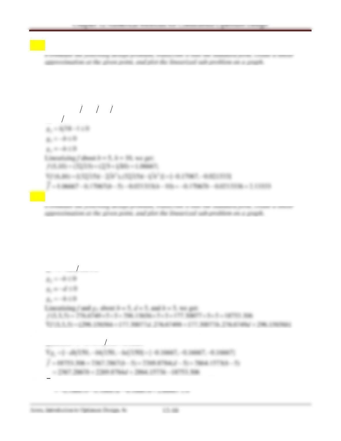
Exercise 2.10 at the point (b, h) = (5, 10) m
Solution:
Substituting the given values the problem is formulated as:
( , ) (32 15)(2 1 )f bh b h= +
1
10 1 0gb= −≤
12.12 _______________________________________________________________________________
Exercise 2.11 at the point, width = 5 m, depth = 5 m, and height = 5 m.
Solution:
Substituting the given values the problem is formulated as:
( , , ) 276.6749 296.15656 177.30077f b d h dh bh bd=++
11 150 0g bdh=−≤
[2367.2867, 2269.8784, 2864.1573]=
1
(5,5,5) 1 5 5 5 150 0.16667g=−×× =
1[ 150, 150, 150] [ 0.16667, 0.16667, 0.16667]g dh bh bd∇=−−−=−−−
18753.306 2367.2867( 5) 2269.8784( 5) 2864.1573( 5)f bdh= + −+ −+ −
2367.2867 2269.8784 2864.1573 18753.306bdh=+ +−
10.16667 0.16667( 5) 0.16667( 5) 0.16667( 5)g bdh= − −− −− −

Chapter 12 Numerical Methods for Constrained Optimum Design
Arora, Introduction to Optimum Design, 4e
12-11
Chapter 12 Numerical Methods for Constrained Optimum Design
12.13 _______________________________________________________________________________
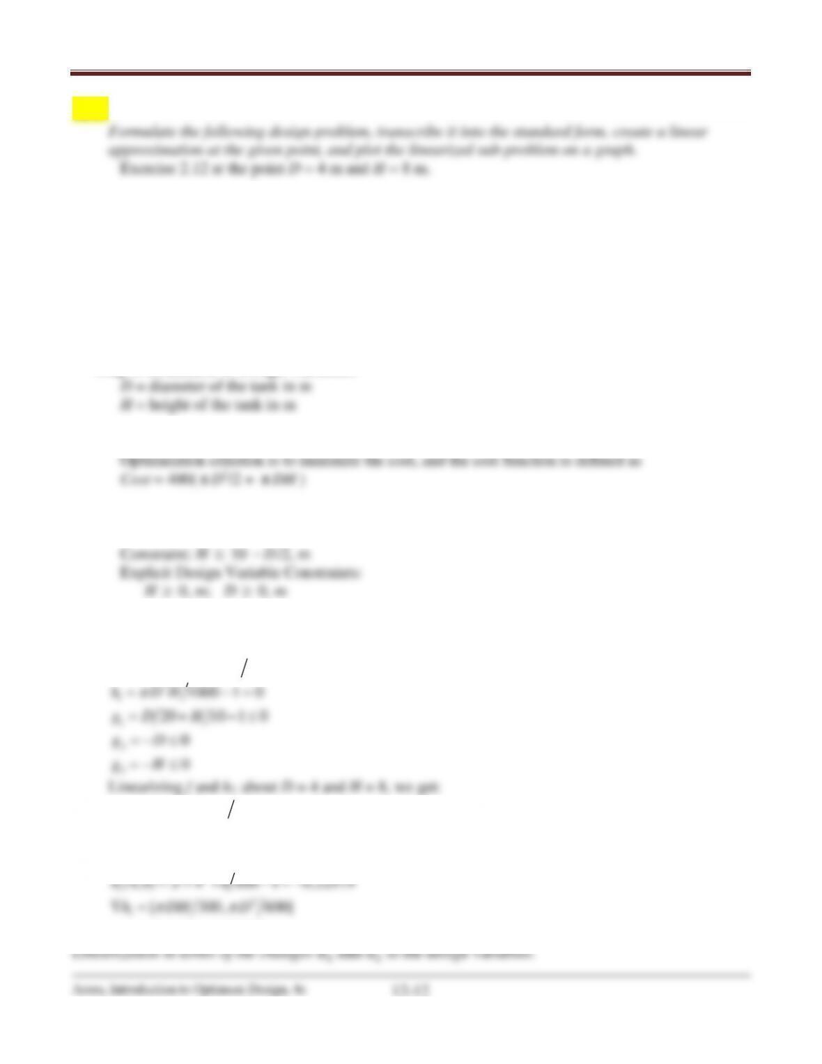
Exercise 2.12
Design a circular tank closed at both ends to have a volume of 250 m3. The fabrication cost is
proportional to the surface area of the sheet metal and is $400/m2. The tank is to be housed in a
shed with a sloping roof. Therefore, height H of the tank is limited by the relation H ≤ (10−D/2),
where D is the tank’s diameter. Formulate the minimum-cost design problem.
Solution:
Step 3: Definition of Design Variables
Step 4: Optimization Criterion
π
π
Step 5: Formulation of Constraints
Constraint:
π
D2H/4 = 250, m3
Substituting the given values, the problem is transcribed into the standard and normalized form as
as:
2
( , ) 400( 2 )f D H D DH
ππ
= +
2
( )
( )
2
(4,8) 400 4 2 4 8 50265.482f
ππ
= + ×× =
(4,8) [400 400 , 400 ]
[15079.645, 5026.548]
f D HD
π ππ
∇= +
=
2
1(4,8) 4 8 600 1 0.32979h
2
1
[ 300, 600]
[0.3351, 0.08378]
h DH D
ππ
∇=
=
Chapter 12 Numerical Methods for Constrained Optimum Design
Arora, Introduction to Optimum Design, 4e
12-13
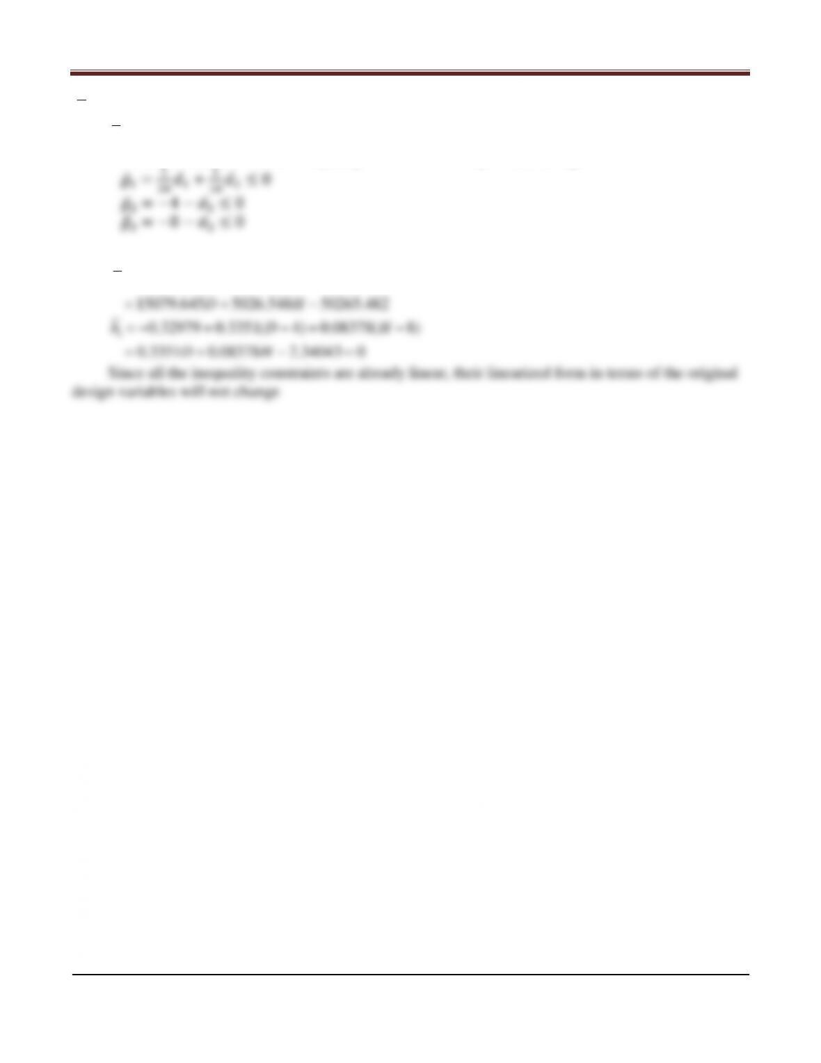
12
50265.482 15079.645 5026.548f dd=++
1 12
0.32979 0.3351 0.08378 0h dd=−+ + =
Similarly linearization of the inequality constraints at the point (4, 8) is given as
Linearization in terms of the original design variables D and H at the point (4, 8):
50265.482 15079.645( 4) 5026.548( 8)
15079.645 5026.548 50265.482
f DH
DH
= + −+ −
= +−
10.32979 0.3351( 4) 0.08378( 8)
0.3351 0.08378 2.34043 0
h DH
DH
=− + −+ −
= + −=
Since all the inequality constraints are already linear, their linearized form in terms of the original
design variables will not change
Chapter 12 Numerical Methods for Constrained Optimum Design
Arora, Introduction to Optimum Design, 4e
12-14
12.14 _______________________________________________________________________________
Exercise 2.13 at the point w = 10 m, d = 10 m, h = 4 m.
Solution:
Substituting the given values the problem is formulated as:
( , , ) 80 120 200f wd h w d h=++
1
1 600 0g wdh=−≤
20gw=−≤
12.15 _______________________________________________________________________________
Exercise 2.14 at the point P1 = 2 and P2 = 1.
Solution:
Substituting the given values the problem is formulated as:
22
12 1 2 1 2
( , ) 2 0.6fPP P P P P=−+ + +
Chapter 12 Numerical Methods for Constrained Optimum Design
Section 12.3 Sequential Linear Programming Algorithm
Note that answers to the exercises in Sections 12.3 are not given in the text because the final results
depend on how the constraints are normalized
12.16 ______________________________________________________________________________
Complete one iteration of the sequential linear programming algorithm for the following problem
(try 50 percent move limits and adjust them if necessary).
Beam design problem formulated in Section 3.8 at the point (b, d) = (250, 300) mm.
Solution:
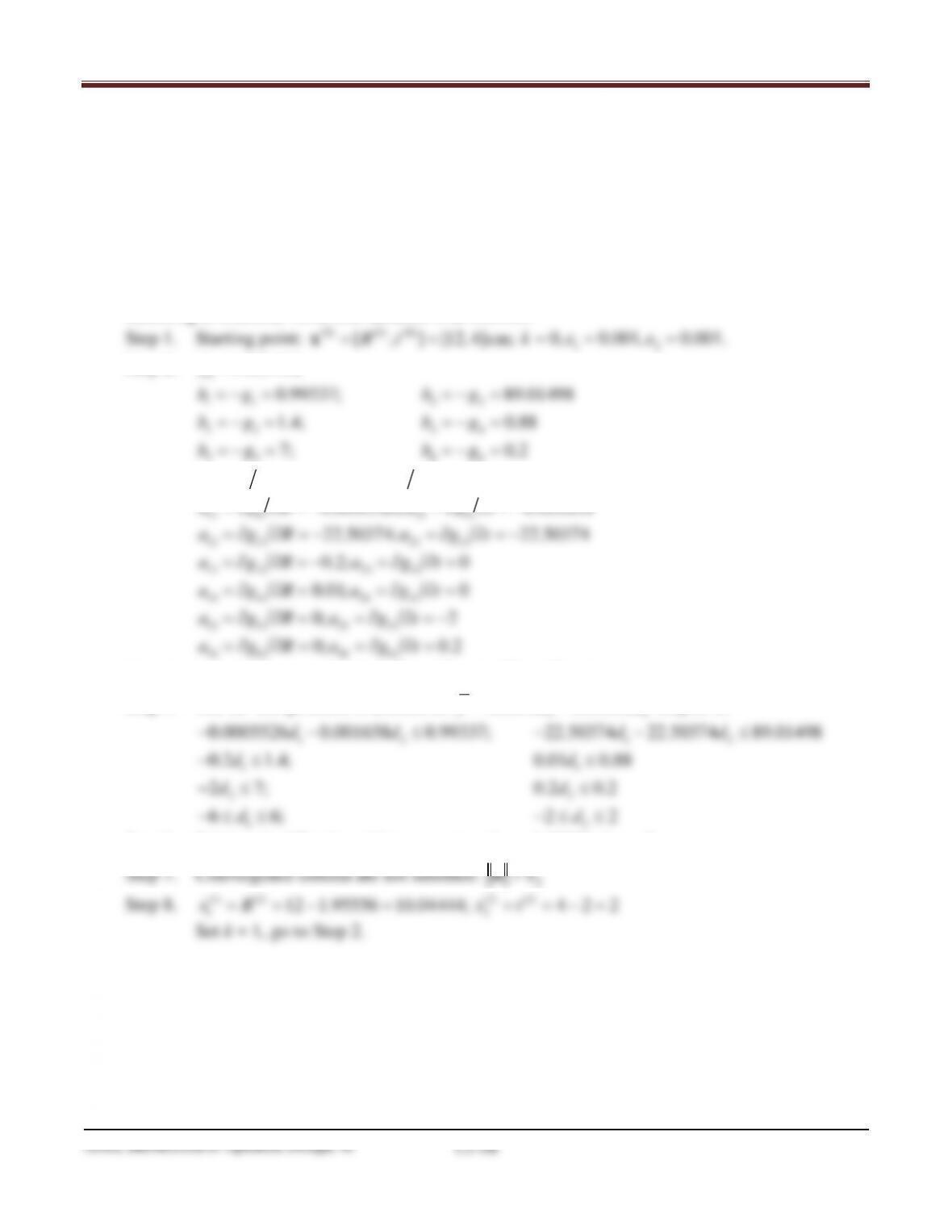
Referring to Exercise 12.3, first iteration is as follows:
(0) (0) (0)
Chapter 12 Numerical Methods for Constrained Optimum Design
12.17 _______________________________________________________________________________
Complete one iteration of the sequential linear programming algorithm for the following problem
(try 50 percent move limits and adjust them if necessary).
Tubular column design problem formulated in Section 2.7 at the point (R, t) = (12, 4) cm. Let
P = 50 kN, E = 210 GPa, l = 500 cm, σa = 250 MPa, and σ = 7850 kg/m3.
Solution:
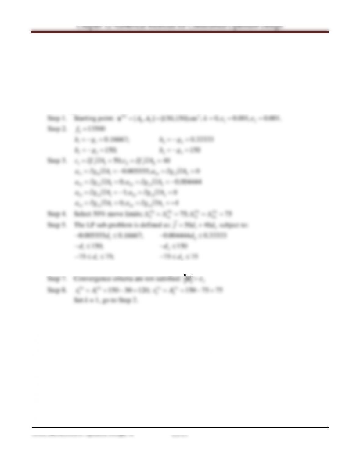
Referring to Exercise 12.4, first iteration is as follows:
(0) (0) (0)
12
Step 2.
0
1183.752f=
55
66
Step 3.
12
98.646; 295.938c fR c ft=∂∂= =∂∂=
11 1 21 1
0.0005526; 0.001658a gR a gt=∂∂=− =∂∂=−
16 6 26 6
Step 4. Select 50% move limits;
(0) (0) (0) (0)
11 22
6; 2
lu lu
∆=∆=∆=∆=
Step 5. The LP sub-problem is defined as:
12
98.646 295.938fd d= +
subject to:
1
2
Step 6. Solving the LP sub-problem, we get:
12
1.95556; 2dd=−=−
12.18 _______________________________________________________________________________
Complete one iteration of the sequential linear programming algorithm for the following problem
(try 50 percent move limits and adjust them if necessary).
Wall bracket problem formulated in Section 4.9.1 at the point (A1, A2) = (150, 150) cm2.
Solution:
Referring to Exercise 12.5, first iteration is as follows:
(0) 2
1
2
Step 6. Solving the LP sub-problem, we get:
12
30; 75dd=−=−
12.19 _______________________________________________________________________________
Exercise 2.1 at the point h = 12 m, A = 4000 m2.
Solution:
Referring to Exercise 12.6, first iteration is as follows:
(0) (0) (0) 2
12
Step 2.
0
11.2f=
Chapter 12 Numerical Methods for Constrained Optimum Design
12.20 _______________________________________________________________________________
Exercise 2.3 at the point (R, H) = (6, 15) cm.
Solution:
Referring to Exercise 12.7, first iteration is as follows:
Step 1. Starting point:
(0) (0) (0)
[ , ] [6,15]cm;RH= =x
12
0, 0.001, 0.001.k
εε
= = =
11
22
33
0.7;bg=−=
44
15bg=−=
55
0.25bg=−=
Step 3.
12
565.487; 113.097c fR c fH=∂∂=− =∂∂ =−
11 1 21 1
12 2 22 2
0.2; 0a gR a gH=∂∂=− =∂∂=
13 3 23 3
0.05; 0a gR a gH=∂∂= =∂∂=
11 22
lu lu
Step 5. The LP sub-problem is defined as:
12
565.487 113.097f dd=−−
subject to:
12
1
0.2 0.2;d−≤
1
0.05 0.7d≤
2
15;d−≤
2
0.05 0.25d≤
1
3 3;d−≤ ≤
2
7.5 7.5d−≤≤
Step 6. Solving the LP sub-problem, we get:
12
3; 1.3736dd= =
2
Step 8.
(1) (1)
1
6 3 9;xR= =+=
(1) (1)
2
15 1.3736 16.3736.xH==+=
Chapter 12 Numerical Methods for Constrained Optimum Design
12.21 _______________________________________________________________________________
Exercise 2.4 at the point R = 2 cm, N = 100.
Solution:
Referring to Exercise 12.8, first iteration is as follows:
(0) (0) (0)
01256.64f= −
11
0.3717;bg=−=
22
3bg=−=
33
Step 3.
12
12.5664; 628.32c fN c fR=∂∂=− =∂∂=−
3
−
11 22
lu lu
Step 5. The LP sub-problem is defined as:
12
12.566 628.32f dd=−−
subject to:
12
Step 7. Convergence criteria are not satisfied:
2
ε
>d
Step 8.
(1) (1)
1100 50 150;xN= = +=
(1) (1)
2
2 0.09156 2.09156.xR==+=