Chapter 10 Numerical Methods for Unconstrained Optimum Design
update(x, xn, d, al, ndv); //call function update() to update the value of xn
fl = funct(xn, nCount); //call function funct() to return the value at a
given value of alpha
update(x, xn, d, aa, ndv);
fa = fu;
update(x, xn, d, au, ndv);
fu = funct(xn, nCount);
}
ab = al+((au–al)/gr);
update(x, xn, d, ab, ndv);
{
case 1:
au = ab;
ab = aa;
case 2:
al = aa;
aa = ab;
Chapter 10 Numerical Methods for Unconstrained Optimum Design
break;
case 3:
al = aa;
au = ab;
fl = fa;
fu = fb;
}
/* calculates the function value
a = value of alpha, input
fVal = function value on return
nC = number of calls for function evaluation
**/
float funct(float xVector[], int *nC)
{
grad[0] = (2*x1)-4-(2*x2);
grad[1] = (4*x2)–(2*x1);
}
void scale(float arrOne[], float arrTwo[], int scalar, int n)
{
for(int i = 0; i < n; i++)
{
arrTwo[i] = scalar*arrOne[i];
}
}

Chapter 10 Numerical Methods for Unconstrained Optimum Design
Arora, Introduction to Optimum Design, 4e
10-43
float sum = 0;
float tNorm = 0;
10.53: x* = (0.0716089, 0.0232635), f * = − 0.0736332, NIT = 8, NFE = 136;
10.55: x* = (0.000010756, 0.0232737), f * = − 0.0116257, NIT = 6, NFE = 103;
10.57: x* = (0.00122397, − 0.00108302, 0.00049956), f * = 0.00000060985, NIT = 41, NFE = 795;
10.59: x* = (3.73284, 0.341954), f * = − 1526.56, NIT = 100, NFE = 1320;
10.61: x* = (0.129072, 0.0129158, 0.0692521, 0.0704564), f * = 0.000374958, NIT = 1000,
Chapter 10 Numerical Methods for Unconstrained Optimum Design
10.63 ______________________________________________________________________________
Consider the following three functions. Minimize f1, f2, and f3 using the program for the steepest-
descent method given in Appendix B. Choose the starting design to be
[1, 1, 2]=x
for all functions. What
do you conclude from observing the performance of the method on the foregoing functions?
222 2 2 2 22 2
1 12321 2 33 12 3
( ) ; 10 100 ; 100 0.1f xxxfx x xf xx x=++ =+ + = ++x
Solutions:
For f1: x* = (0.000198483, 0.000198483, 0.000396967), f
*
1
= 2.36374E−07, NIT = 1, NFE = 23;
*
To get the solutions in one iteration for f2 and f3, the following transformations are suggested.
(With these, the condition number becomes one):
20 0
0 0 200
12 0 0
0 0 1 200
For f3:
200 0 0
0 2 0,
0 0 0.2
=
H
1 200 0 0
0 12 0
0 0 1 0.2
=
xy
Arora, Introduction to Optimum Design, 4e
10-45
10.64 ______________________________________________________________________________
Calculate the gradient of the following functions at the given points by the forward, backward, and
central difference approaches with a 1 percent change in the point and compare them with the exact
gradient.
22
1 1 2 12
( ) 12.096 21.504 1.7321 ;f x x xx= + −−x
starting point
[5, 6]=x
22 2
2 21 1
( ) 50( x ) (2 x ) ;fx= − +−x
starting point
[1, 2]=x
222
3 1 2 3 12 23
( ) 2 2 2x x 2x x ;f xxx=+++ +x
starting point
[1, 2, 3]=x
Solution:
( ) 12.096 21.504 1.7321 ;f x x xx= + −−x
[5, 6]=x
22
1 1 2 12
1 1 11 2 1 2
2. Forward Difference Approach
11 1 1
12 1 1
[ (5,6.06) (5,6)] 0.06 15.50 0.06 258.3382fx f f∂∂= − = =
3. Backward Difference Approach
11 1 1
[ (5,6) (4.95,6)] 0.05 5.9312 0.05 118.6fx f f∂∂= − = =
12 1 1
4. Central Difference Approach
11 1 1
[ (5.05,6) (4.95,6)] 0.10 11.923 0.10 119.2fx f f∂∂= − = =
22 2
( ) 50( x ) (2 x ) ;fx= − +−x
2 21 1
2 2 12 2 2 1 1 1 21
2. Forward Difference Approach
21 2 2
[ (1.01, 2) (1, 2)] 0.01 2.0097 0.01 200.97fx f f∂ ∂= − =− =−
22 2 2
4. Backward Difference Approach
21 2 2
[ (1, 2) (0.99, 2)] 0.01 2.0299 0.01 202.99fx f f∂ ∂= − =− =−
22 2 2
4. Central Difference Approach
21 2 2
[ (1.01, 2) (0.99, 2)] 0.02 4.0396 0.02 201.98fx f f∂ ∂= − =− =−
22 2 2
Chapter 10 Numerical Methods for Unconstrained Optimum Design
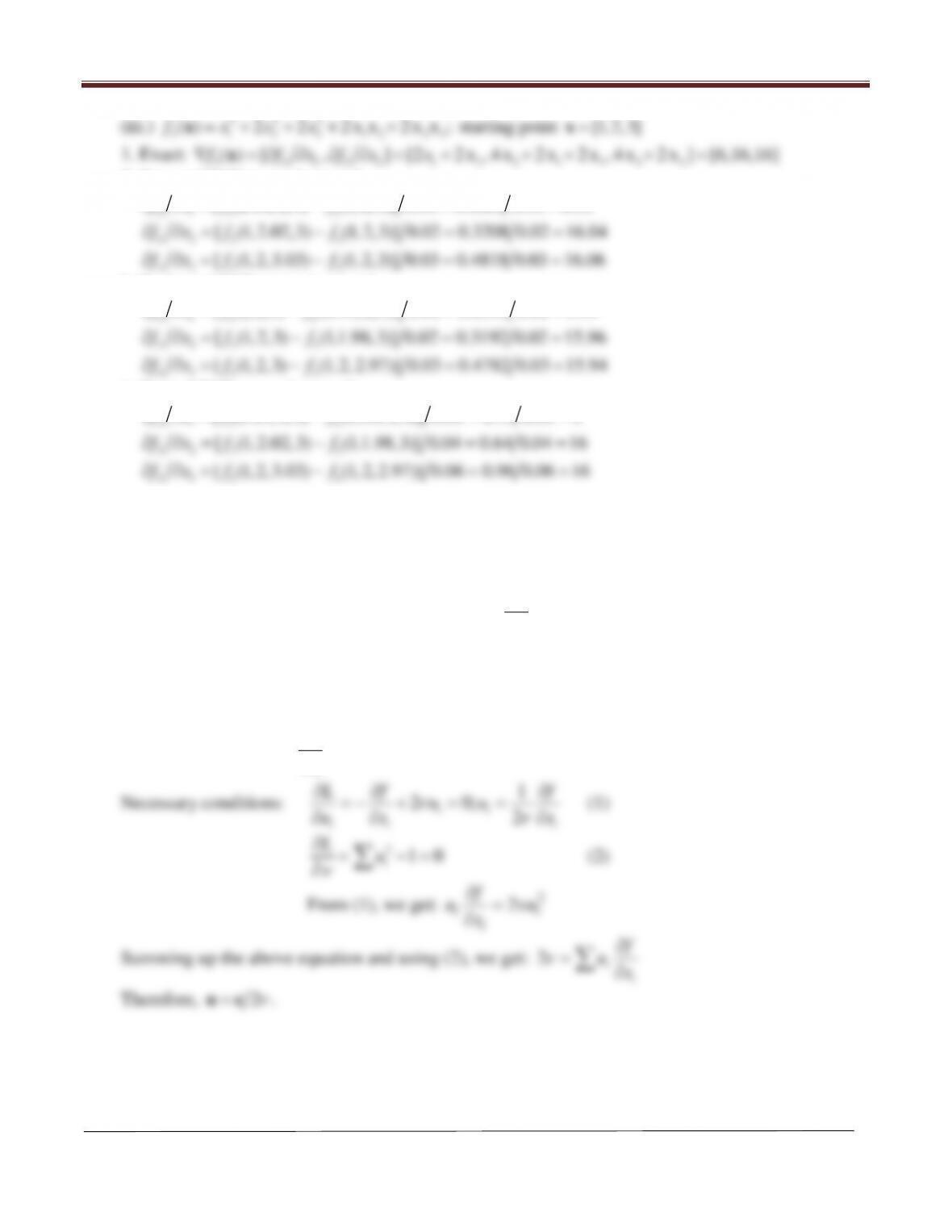
222
3 3132 1 221332
2. Forward Difference Approach
31 3 3
[ (1.01, 2,3) (1, 2,3)] 0.01 0.0601 0.01 6.01fx f f∂ ∂= − = =
33 3 3
3. Backward Difference Approach
31 3 3
[ (1, 2,3) (0.99, 2,3)] 0.01 0.0599 0.01 5.99fx f f∂ ∂= − = =
[ (1, 2,3) (1, 2, 2.97)] 0.03 0.4782 0.03 15.94fx f f∂∂= − = =
[ (1, 2,3.03) (1, 2, 2.97)] 0.06 0.96 0.06 16fx f f∂∂= − = =

Chapter 10 Numerical Methods for Unconstrained Optimum Design
Arora, Introduction to Optimum Design, 4e
10-47
Section 10.7 Search Direction Determination: Conjugate Gradient Method
10.66______________________________________________________________________________
Answer True or False.
Solution:
1. The conjugate gradient method usually converges faster than the steepest-descent method. True
3. Conjugate directions are normal to each other. False
5. The conjugate direction at the kth point is orthogonal to the gradient of the cost function at the
(k−1)th point. False
Chapter 10 Numerical Methods for Unconstrained Optimum Design
Arora, Introduction to Optimum Design, 4e
10-48
10.67 ______________________________________________________________________________
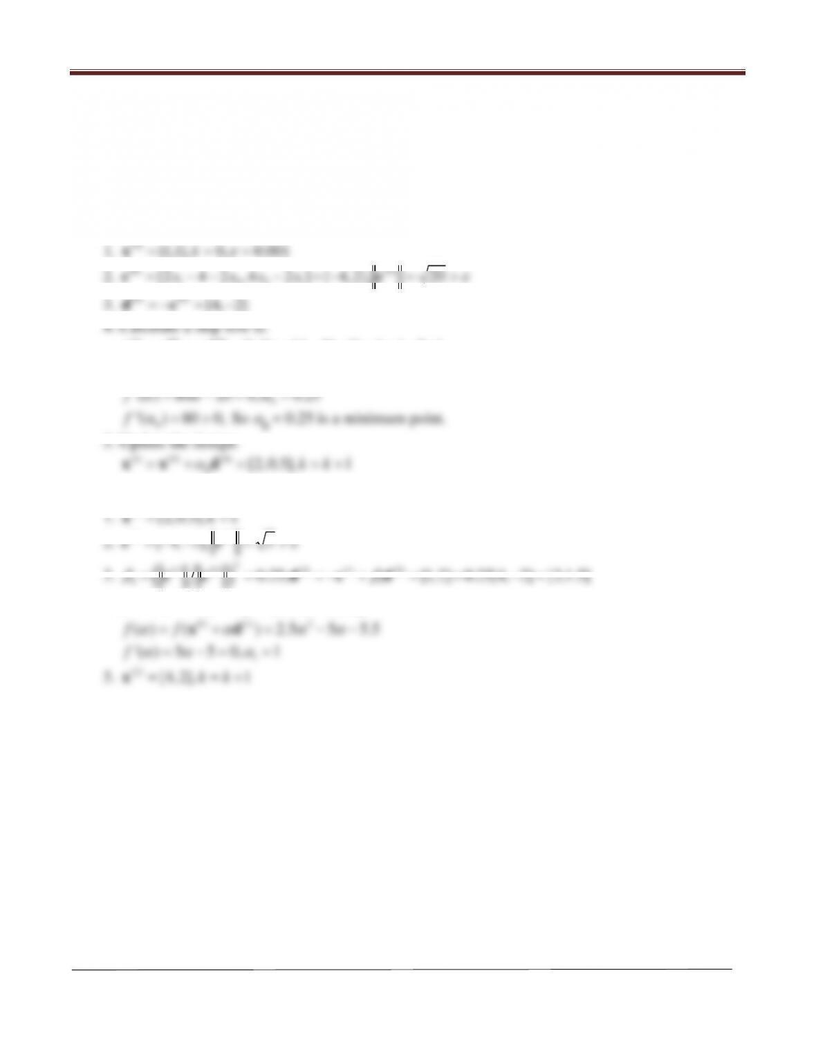
For the following function, complete two iterations of the conjugate gradient method starting from
the given design point.
22
1 2 1 2 1 12
(, ) 2 4 2 ;f x x x x x xx=+ −−
starting point,
[1, 1]=x
Solution:
Iteration 1:
1.
(0) [1,1], 0, 0.001k
ε
= = =x
2.
(0) (0)
1 22 1
[2 4 2 , 4 2 ] [ 4, 2], 20x xx x
ε
= −− − =− = >cc
3.
(0) (0) [4, 2]=−=−dc
(1) (0) (0)
[1,1] [4, 2] [1 4 ,1 2 ]
α α αα
= + = + −=+ −xx d
(0) (0) 2
( ) ( ) 40 20 3ff
α α αα
= + = −−xd
0[2, 0.5], 1kk
Iteration 2:
(1) [2, 0.5], 1k= =x
3.
( )
2
(1) (0) (1) (1) (0)
11
0.25; [1, 2] 0.25[4, 2] [2,1.5]
ββ
= = =− + = + −=cc d c d
4.
(2) (1) (1)
[2 2 , 0.5 1.5 ];
α αα
=+=+ +xx d
(1) (1) 2
Chapter 10 Numerical Methods for Unconstrained Optimum Design
Arora, Introduction to Optimum Design, 4e
10-49
10.68 ______________________________________________________________________________
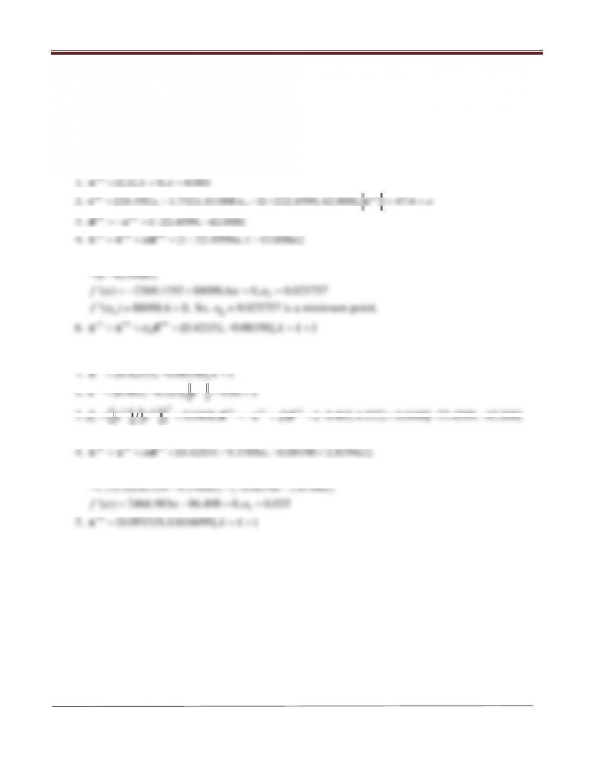
For the following function, complete two iterations of the conjugate gradient method starting from
the given design point.
22
12 1 2 1 2
( , ) 12.096 21.504 x 1.7321 ;fxx x x x= + −−
starting point,
[1, 1]=x
Solution:
Iteration 1:
1.
(0) [1,1], 0, 0.001k
ε
= = =x
2.
(0) (0)
12
[24.192 1.7321, 43.008 x 1] [22.4599, 42.008], 47.6x
ε
= − −= = >cc
3.
(0) (0) [ 22.4599, 42.008]=−=− −dc
(1) (0) (0)
(0) (0) 2 2
( ) ( ) 12.096(1 22.4599 ) 21.504(1 42.008 ) 1.7321(1 22.4599 )
(1 42.008 )
ff
αα α α α
α
=+= − + − − −
−−
xd
0
‘( ) 2269.1192 88098.6 0, 0.025757f
α αα
=−+==
0
‘‘( ) 88098.6 0,f
α
= >
So,
α
0 = 0.025757 is a minimum point.
6.
(1) (0) (0)
0
[0.42151, 0.08198], 1kk
α
=+= − =+xx d
Iteration 2:
(1) [0.42151, 0.08198], 1k=−=x
3.
( )
2
(1) (0) (1) (1) ( 0)
11
0.0406; [ 8.465, 4.525] 0.0406[ 22.4599, 42.008]
ββ
= = =−+ =− + − −cc d c d
[ 9.3769, 2.8194]= −
(2) (1) (1)
(1) (1) 2 2
( ) ( ) 12.096(0.42151 9.3769 ) 21.504( 0.08198 2.8194 )
1.7321(0.42151 9.3769 ) ( 0.08198 2.8194 )
ff
αα α α
αα
=+= − + − +
− − −− −
xd
Chapter 10 Numerical Methods for Unconstrained Optimum Design
10.69 ______________________________________________________________________________
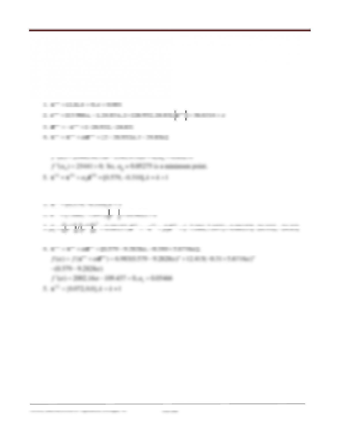
For the following function, complete two iterations of the conjugate gradient method starting from
the given design point.
22
12 1 2 1
( , ) 6.983 12.415 ;fxx x x x=+−
starting point,
[2,1]=x
Solution:
Iteration 1:
1.
(0) [2,1], 0, 0.001k
ε
= = =x
2.
(0) (0)
12
[13.966 1, 24.83 x ] [26.932, 24.83], 36.6314x
ε
=−= =>cc
3.
(0) (0) [ 26.932, 24.83]=−=− −dc
(1) (0) (0)
(0) (0) 2 2
( ) ( ) 6.983(2 26.932 ) 12.415(1 24.83 ) (2 26.936 )ff
αα α α α
= + = − + − −−xd
0
‘( ) 25441.4173 1341.97325 0, 0.05275f
αα α
= −==
0
‘‘( ) 25441 0;f
α
= >
So,
α
0 = 0.05275 is a minimum point.
5.
(1) (0) (0)
0[0.579, 0.310], 1kk
α
=+= − =+xx d
Iteration 2:
(1) [0.579, 0.310], 1k=−=x
3.
( )
2
(1) (0) (1) (1) (0)
11
0.08157; [ 7.086,7.697] 0.08157[ 26.932, 24.83]
ββ
= = =−+ =− + − −cc d c d
[ 9.2828,5.6716]= −
(2) (1) (1) [0.579 9.2828 , 0.310 5.6716 ];
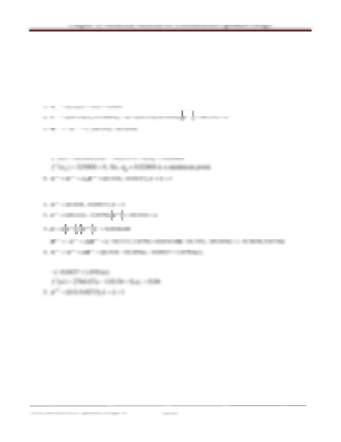
10.70______________________________________________________________________________
For the following function, complete two iterations of the conjugate gradient method starting from
the given design point.
22
12 1 2 2
( , ) 12.096 21.504 ;fxx x x x=+−
starting point,
[1, 2]=x
Solution:
Iteration 1:
(0) [1, 2], 0, 0.001k
2.
(0) (0)
12
[24.192 , 43.008 x 1] [24.192,85.016], 88.391x
ε
= −= = >cc
(0) (0) [ 24.192, 85.016]=−=− −dc
4.
(1) (0) (0) [1 24.192 , 2 85.016 ]
α αα
=+=− −xx d
(0) (0) 2 2
( ) ( ) 12.096(1 24.192 ) 21.504(2 85.016 ) (2 85.016 )ff
αα α α α
= + = − + − −−xd
0
‘( ) 325008.23 7812.973 0, 0.02404f
αα α
= −==
0
‘‘( ) 325008 0,f
α
= >
So,
α
0 = 0.02404 is a minimum point.
5.
(1) (0) (0)
0[0.418, 0.0437], 1kk
α
=+= − =+xx d
Iteration 2:
1.
(1) [0.418, 0.0437], 1k=−=x
2.
(1) (1)
[10.112, 2.879], 10.514
ε
=−=>cc
3.
( )
2
(1) (0)
1
0.014148
β
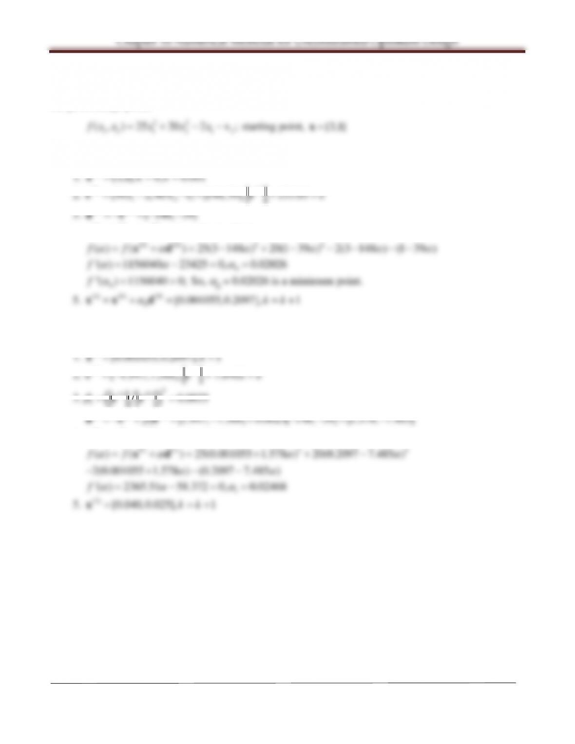
= =cc
(1) (1) (0)
Arora, Introduction to Optimum Design, 4e
10-52
10.71______________________________________________________________________________
For the following function, complete two iterations of the conjugate gradient method starting from
the given design point.
12 1 2 1 2
Solution:
Iteration 1:
(0) [3,1], 0, 0.001k
2.
(0) (0)
12
[50 2, 40 x 1] [148,39], 153.05x
ε
= − −= = >cc
(0) (0) [ 148, 39]=−=− −dc
4.
(1) (0) (0)
[3 148 ,1 39 ]
α αα
=+=− −xx d
(0) (0) 2 2
( ) ( ) 25(3 148 ) 20(1 39 ) 2(3 148 ) (1 39 )ff
α α α α αα
= + = − + − − − −−xd
0
‘( ) 1156040 23425 0, 0.02026f
αα α
= −==
0
‘‘( ) 1156040 0;f
α
= >
So,
α
0 = 0.02026 is a minimum point.
5.
(1) (0) (0)
0[0.001055,0.2097], 1kk
α
=+= =+xx d
Iteration 2:
Iteration 2:
(1) [0.001055,0.2097], 1k= =x
3.
( )
2
(1) (0)
1
0.0025
β
= =cc
(1) (1) (0)
1
[1.947, 7.388] 0.0025[ 148, 39] [1.578, 7.485]
β
=−+ = − + − −= −dc d
5.
(2) (1) (1)
[0.001055 1.578 ,0.2097 7.485 ];
α αα
=+= + −xx d
(1) (1) 2 2
( ) ( ) 25(0.001055 1.578 ) 20(0.2097 7.485 )
ff
αα α α
=+= + + −
xd