Chapter 10 Numerical Methods for Unconstrained Optimum Design
10.72 ______________________________________________________________________________
For the following function, complete two iterations of the conjugate gradient method starting from
the given design point.
222
1 2 3 1 2 3 12 23
(,,x) 222 2;fxx xxxxxxx=+++ +
starting point,
[1, 1,1]=x
Solution:
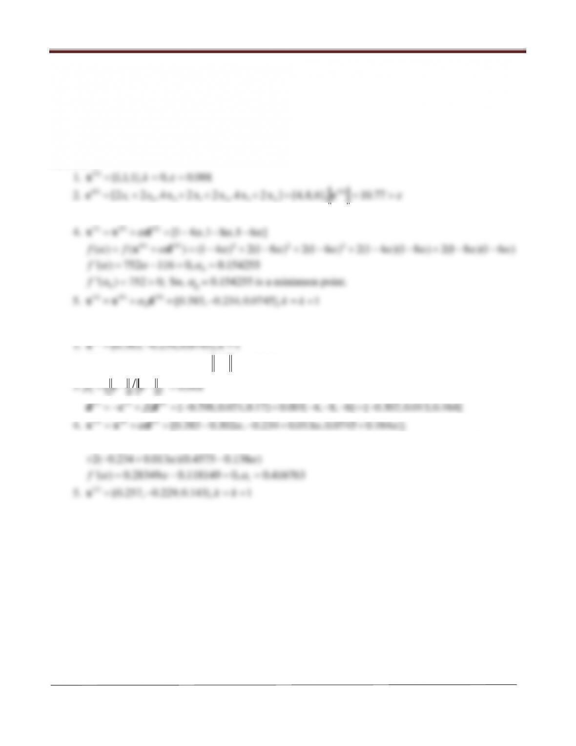
Iteration 1:
(0) [1,1,1], 0, 0.001k
1221332
3.
(0) (0) [4,8,6]=− =−−−dc
(1) (0) (0)
0
Iteration 2:
(1) [0.383, 0.234,0.0745], 1k=−=x
2.
(1) (1)
[0.298, 0.021, 0.17], 0.3437
ε
= −− = >cc
2
(1) (0)
Chapter 10 Numerical Methods for Unconstrained Optimum Design
10.73 ______________________________________________________________________________
For the following function, complete two iterations of the conjugate gradient method starting from
the given design point.
2 2 22 22
12 1 2 12 2 12 2 1 2
( , ) 8 8 80 20 100 80 20 100 5 x 5 x ;fxx x x xx x xx x= + − +− + + ++ + − −
starting point,
[4, 6]=x
Solution:
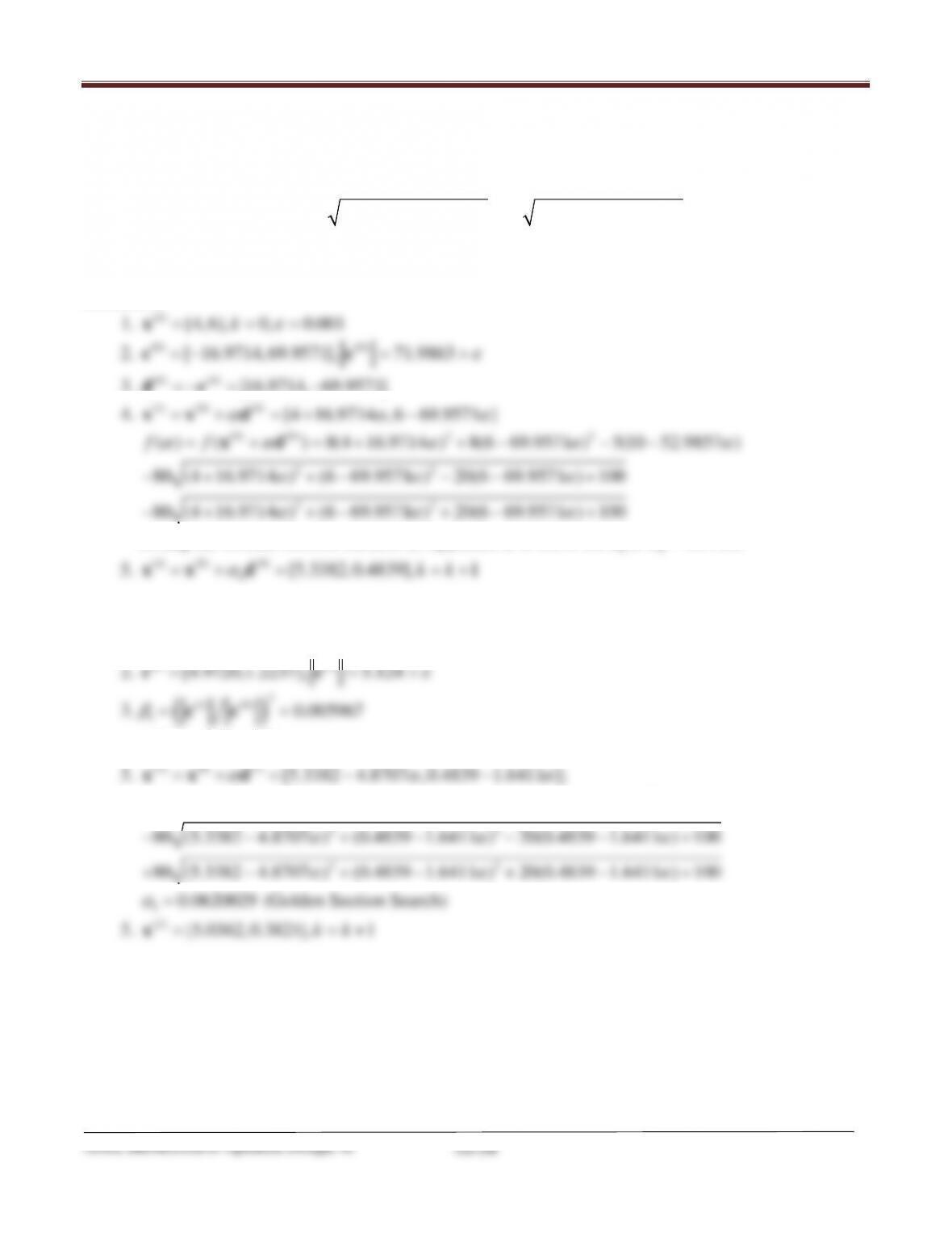
Iteration 1:
(0) [4,6], 0, 0.001k
3.
(0) (0) [16.9714, 69.9571]=−= −dc
(1) (0) (0)
22
80 (4 16.9714 ) (6 69.9571 ) 20(6 69.9571 ) 100
αα α
−++−+−+
(Using the Golden Section Method in Appendix B to solve for 0
α
);
00.07885
α
=
(1) (0) (0)
0
Iteration 2:
1.
(1) [5.3382,0.4839], 1k= =x
(1) (1)
3.
( )
2
(1) (0)
1
0.005967
β
= =cc
(1) (1) (0)
1
[ 4.9720, 1.2237] 0.005967[16.9714, 69.9571] [ 4.8707, 1.6411]
β
=−+ =− − + − =− −dc d
(2) (1) (1) [5.3382 4.8707 ,0.4839 1.6411 ];
10.74 ______________________________________________________________________________
For the following function, complete two iterations of the conjugate gradient method starting from
the given design point.
2 2 22 22
12 1 2 12 2 12 2 1 2
( , ) 9 9 100 20 100 64 16 64 5 x 41x ;fxx x x xx x xx x= + − +− + − ++ + − −
starting point,
[5, 2]=x
Solution:
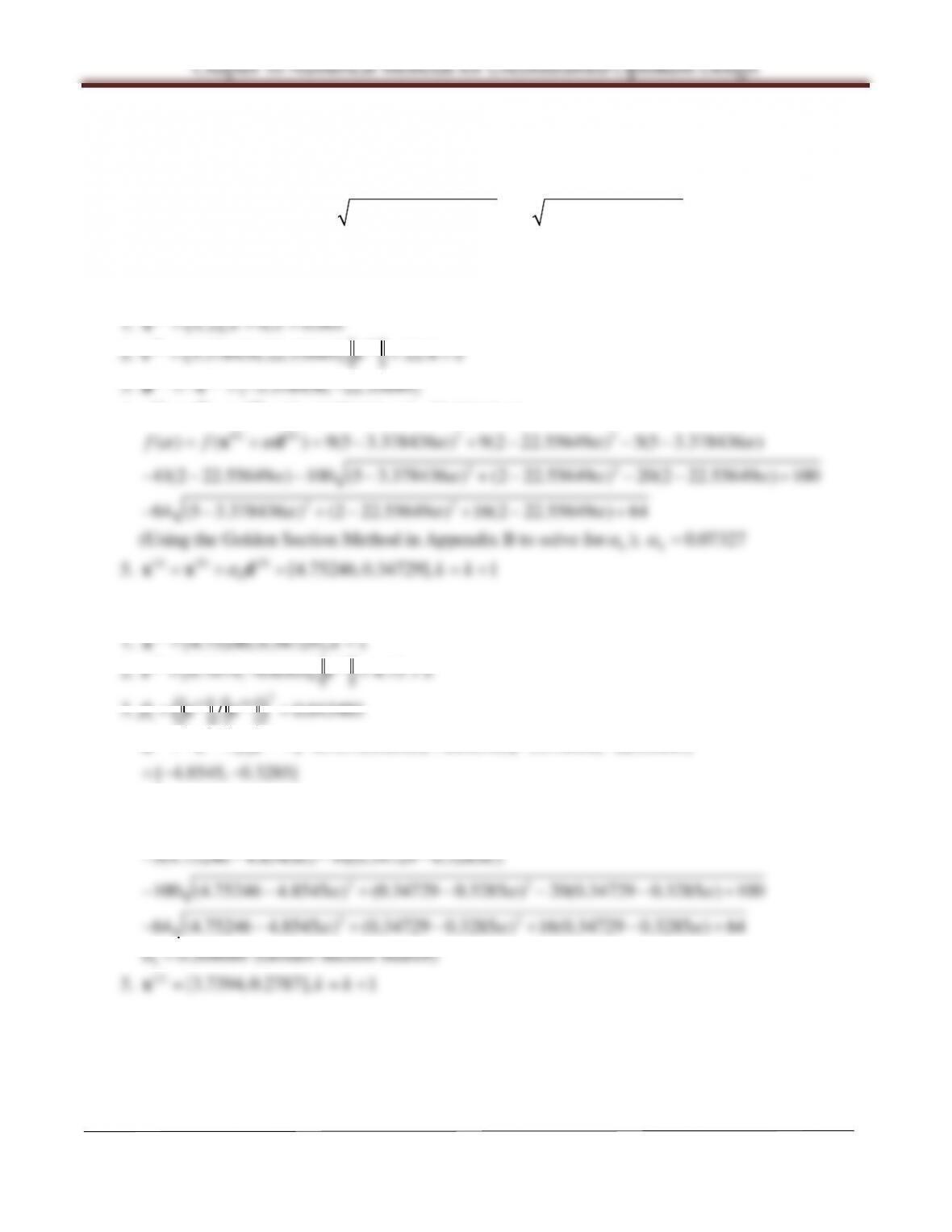
Iteration 1:
(0) [5,2], 0, 0.001k
2.
(0) (0)
[3.378436, 22.55649], 22.8
ε
= = >cc
3.
(0) (0)
[ 3.378436, 22.55649]=−=− −dc
4.
(1) (0) (0) [5 3.378436 , 2 22.55649 ]
α αα
=+=− −xx d
(0) (0) 2 2
22
22
( ) ( ) 9(5 3.378436 ) 9(2 22.55649 ) 5(5 3.378436 )
41(2 22.55649 ) 100 (5 3.378436 ) (2 22.55649 ) 20(2 22.55649 ) 100
64 (5 3.378436 ) (2 22.55649 ) 16(2 22.55649 ) 64
ff
αα α α α
α αα α
αα α
= + =− +− −−
−−−− +− −−+
− − +− + − +
xd
(Using the Golden Section Method in Appendix B to solve for 0
α
);
00.07327
α
=
5.
(1) (0) (0)
0[4.75246,0.34729], 1kk
α
=+= =+xx d
Iteration 2:
(1) [4.75246,0.34729], 1k= =x
3.
( )
2
(1) (0)
1
0.043403
β
= =cc
(1) (1) (0 )
1[ 4.7079,0.6505] 0.043403[ 3.378436, 22.55649]
[ 4.8545, 0.3285]
β
=−+ =− + − −
=−−
dc d
4.
(2) (1) (1)
[4.75246 4.8545 , 0.34729 0.3285 ];
α αα
=+= − −xx d
(1) (1) 2 2
22
2
( ) ( ) 9(4.75246 4.8545 ) 9(0.34729 0.3285 )
5(4.75246 4.8545 ) 41(0.34729 0.3285 )
100 (4.75246 4.8545 ) (0.34729 0.3285 ) 20(0.34729 0.3285 ) 100
64 (4.75246 4.8545 ) (0.34729 0.3285
ff
αα α α
αα
αα α
αα
=+= − + −
− −− −
− − +− − − +
− − +−
xd
2
) 16(0.34729 0.3285 ) 64
α
+ −+
1
0.208686
α
=
(Golden Section Search)
5.
(2)
[3.7394,0.2787], 1kk= = +x
Chapter 10 Numerical Methods for Unconstrained Optimum Design
10.75 ______________________________________________________________________________
For the following function, complete two iterations of the conjugate gradient method starting from
the given design point.
22 2
12 2 1 1
( , ) 100( x ) (1 x ) ;fxx x= − +−
starting point,
[5, 2]=x
Solution:
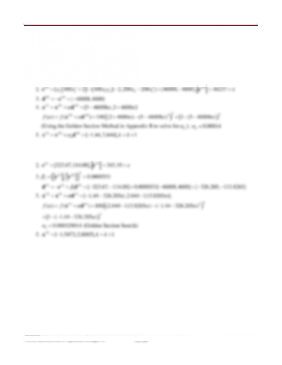
Iteration 1:
1.
(0) [5,2], 0, 0.00001k
ε
= = =x
(0) 2 2 (0)
0
Iteration 2:
1.
(1)
[ 1.44, 2.644], 1k=−=x
(1) (1)
Arora, Introduction to Optimum Design, 4e
10-57
10.76 ______________________________________________________________________________
For the following function, complete two iterations of the conjugate gradient method starting from
the given design point.
22 4 4
123 4 1 2 3 4 2 3 1 4
( , , , x ) (x 10 x ) 5(x x ) (x 2 x ) 10(x x ) ;fxx x =− + − +− + −
starting point,
[1,2,3,4]=x
Solution:
Iteration 1:
(0)
2.
(0) 3 3 3
1 2 14 1 2 23 34 23
[2( 10 x ) 40(x x ) , 20(x 10 x ) 4(x 2 x ) ,10(x x ) 8(x 2 x ),x=−+−−−+− −−−c
3 (0)
34 14
10(x x ) 40(x x ) ] [ 1118,124,502,1090], 1645
ε
− −− − =− = >c
(0) (0) [1118, 124, 502, 1090]=−= −−−dc
4.
(1) (0) (0) [1 1118 , 2 124 ,3 502 , 4 1090 ]
α ααα α
=+=+ − − −xx d
(0) (0) 2 2 4 4
( ) ( ) (2358 19) 5(588 1) (880 4) 10(2208 3)ff
αα α αα α
= + = − + −+ − + −xd
(Using the Golden Section Method in Appendix B to solve for 0
α
);
00.001854
α
=
5.
(1) (0) (0)
0[3.0728,1.7701, 2.06929,1.97914], 1kk
α
=+= =+xx d
Iteration 2:
(1)
2.
(1) (1)
[23.068, 239.418,107.193, 53.226], 268.66
ε
= −=>cc
3.
( )
2
(1) (0)
10.0266731
β
= =cc
(1) (1) (0 )
1
[ 23.068, 239.418, 107.193,53.226]
0.0266731[1118, 124, 502, 1090] [6.7524, 242.7255, 120.5829, 24.1524]
β
=−+ =− − −
+ −−− = − −
dc d
6.
(2) (1) (1) [3.0728 6.7524 ,1.7701 242.7255 ,
α αα
=+= + −xx d
2.06929 120.5829 ,1.97914 24.1524 ]
αα
−+
(1) (1) 2 2
44
( ) ( ) ( 14.6282 2434.0074 ) 5(0.09015 144.7353 )
( 2.36848 1.5597 ) 10(1.09366 17.4 )
ff
αα α α
αα
=+=− + + −
+− − + −
xd
1
0.0059028
α
=
(Golden Section Search)
5.
(2) [3.113, 0.3374,1.3574, 2.1214], 1kk= = +x
Chapter 10 Numerical Methods for Unconstrained Optimum Design
10.77 ______________________________________________________________________________
Write a computer program to implement the conjugate gradient method (or, modify the steepest-
descent program given in Appendix B). Solve Exercises 10.52 to 10.61 using your program.
Solutions:
The solutions were obtained using the following program, written in C++.
void update(float x[], float xwrk[], float d[], float a, int n);
void printStuff(int currCount, float x[], float alph, float grad[], float f, int
ndv);
int main()
{
float delta = 0.05; // * modify this value for the required delta for
float x[2] = {1, 1}; // * modify this array to hold design variable vector
float d[2] = {0, 0}; // * modify this array to hold the direction vector
float c[2] = {0, 0}; // holds the gradient vector
float wrk[2] = {0, 0}; // vector to hold temporary values
float alpha = 0; // holds the value of alpha at the minimum
Chapter 10 Numerical Methods for Unconstrained Optimum Design
}
for(int k = 1; k <= noc; k++)
{
cmag1 = tNorm(c, ndv);
printStuff(k, x, alpha, c, f, ndv);
grad(x, c);
cmag2 = tNorm(c, ndv);
beta = pow(cmag2/cmag1, 2);
scale(c, d, beta, ndv);
}
}
if(nocActual >= noc)
{
e = convergence parameter
f = optimum value of the function on return
n = number of function evaluations on return
**/
void goldenIntervalSearch(float x[], float xn[], float d[], float *a, float delta,
float epsilon, float *f, int *nCount, int ndv)
{
Chapter 10 Numerical Methods for Unconstrained Optimum Design
float delta1 = delta; //holds optimal value of delta, initially
set to passed value
float al = 0; //lower bound of alpha
fl = funct(xn, nCount); //call function funct() to return the value
at a given value of alpha
update(x, xn, d, aa, ndv);
fa = funct(xn, nCount);
update(x, xn, d, au, ndv);
fu = funct(xn, nCount);
}
ab = al+((au–al)/gr);
update(x, xn, d, ab, ndv);
fb = funct(xn, nCount);
//refine the interval of uncertainty further
{
case 1:
au = ab;
Chapter 10 Numerical Methods for Unconstrained Optimum Design
aa = al+((1–1/gr)*(au–al));
update(x, xn, d, aa, ndv);
fa = funct(xn, nCount);
break;
case 2:
al = aa;
aa = ab;
case 3:
al = aa;
au = ab;
fl = fa;
fu = fb;
}
/* calculates the function value
a = value of alpha, input
fVal = function value on return
nC = number of calls for function evaluation
**/
float funct(float xVector[], int *nC)
{
Chapter 10 Numerical Methods for Unconstrained Optimum Design
}
void scale(float arrOne[], float arrTwo[], int scalar, int n)
{
for(int i = 0; i < n; i++)
{
arrTwo[i] = –1*arrOne[i]+scalar*arrTwo[i];
}
}
float tNorm(float vec[], int n)
void update(float x[], float xwrk[], float d[], float a, int n)
{
}
void printStuff(int currCount, float x[], float alph, float grad[], float f, int
ndv)
{
cout<<“Iteration number: “<<currCount<<” Function value: “<<f<<” Alpha value:
“<<alph<<“\n”;
cout<<“Norm of gradient vector: “<<tNorm(grad, ndv)<<“\n”;
}
____________________________________________________________________________________
10.53: x* = (0.0716066, 0.0232642), f * = − 0.0736332, NIT = 8, NFE = 125;
10.55: x* = (0.00000998224, 0.0232725), f * = − 0.0116257, NIT = 6, NFE = 96;
10.57: x* = (0.000494682, -0.000290992, 0.000167161), f * = 0.0, NIT = 18, NFE = 388;
10.59: x* = (3.73312, 0.341153), f * = −1526.56, NIT = 16, NFE = 227;
10.61: x* = (0.0488862, 0.00489234, 0.0264347, 0.0264981), f * = 0.00000783204, NIT = 80,

Chapter 10 Numerical Methods for Unconstrained Optimum Design
Note: In the solution of Exercises 10.78 – 10.87(Exercises 10.52 – 10.61, respectively), use Excel–
Solver.
Solution:
An example is shown for the solution of Exercise 10.52 (Exercise 10.78)
Microsoft Excel 15.0 Answer Report
Worksheet: [Book2]Sheet1
Report Created: 7/30/2014 4:11:04 PM
Result: Solver found a solution. All Constraints and optimality conditions are satisfied.
Solver Engine
Engine: GRG Nonlinear
Solution Time: 0.016 Seconds.
Iterations: 3 Subproblems: 0
Solver Options
Max Time Unlimited, Iterations Unlimited, Precision 0.000001
Convergence 0.0001, Population Size 100, Random Seed 0, Derivatives Central
Max Subproblems Unlimited, Max Integer Sols Unlimited, Integer Tolerance 1%
Objective Cell (Min)
Cell
Name
Original
Value
Final
Value
$C$
6
function
:
-3
-8
Variable Cells
Cell
Name
Original
Value
Final
Value
Intege
r
$C$
3
x1
1
4
Contin
$C$
4
x2
1
2
Contin
x1 1
x2 1
function: -3
x1 4
x2 2
function: -8

Chapter 10 Numerical Methods for Unconstrained Optimum Design
Arora, Introduction to Optimum Design, 4e
10-64
Constraints
NONE