Accounting Chapter 9 Homework Cornerstone Exercise 911 Using The Standard Mix

9-1

CHAPTER 9

STANDARD COSTING:

A FUNCTIONAL-BASED CONTROL APPROACH

DISCUSSION QUESTIONS

1. Standard costs are essentially budgeted

amounts on a per-unit basis. Unit standards

serve as inputs in building budgets.

2. The quantity decision is determining how

much input should be used per unit of out-

put. The pricing decision determines how

much should be paid for the quantity of input

used.

3. Historical experience is often a poor choice

for establishing standards because the his-

torical amounts may include more inefficien-

cy than is desired.

4. Ideal standards are perfection standards,

representing the best possible outcomes.

Currently attainable standards are standards

that are challenging but allow for inefficien-

cy. Currently attainable standards are often

chosen because many feel they tend to mo-

tivate rather than frustrate.

5. By identifying standards and assessing de-

viations from the standards, managers can

locate areas where change or corrective be-

havior is needed.

6. Managers generally tend to have more control

over the quantity of an input used, rather than

the price paid per unit of input.

7. The materials price variance is often com-

puted at the point of purchase rather than

issuance because it provides control infor-

mation sooner. If the variance is computed

at the point of issuance and a problem is de-

tected, this problem could have been ongo-

ing for weeks or months (depending on how

long the direct materials were in inventory

before being used).

8. Disagree. A direct materials usage variance

can be caused by factors beyond the control

of the production manager (e.g., purchase of

a lower quality of direct materials than nor-

mal).

9. Disagree. Using higher-priced workers to

perform lower-skilled tasks is an example of

an event that will create a direct labor rate

variance that is controllable.

10. Inefficient direct labor, machine downtime,

bored workers, and poor quality direct mate-

rials are possible causes of an unfavorable

direct labor efficiency variance.

11. Part of a variable overhead spending vari-

ance can be caused by inefficient use of

overhead resources.

12. The volume variance is caused by the actual

volume differing from the expected volume

used to compute the predetermined standard

fixed overhead rate. If the actual volume is

different from the expected volume, then the

company has either lost or earned a contribu-

tion margin. The volume variance signals this

outcome. If the variance is large, then the

loss or gain is large since the volume vari–

ance understates the effect.

13. Control limits indicate how large a variance

must be before it is judged to be material

and the process is out of control. Current

practice sets the control limits subjectively

and bases them on past experience, intui-

tion, and judgment.

14. All three approaches break the total overhead

variance into component variances. The four-

variance approach divides overhead into fixed

and variable categories (based on unit-level

behavior). It computes the variable overhead

spending and efficiency variances and the

fixed spending and volume variances. The

three-variance approach computes the

spending variance (the sum of the fixed and

variable spending variances of the four–

variance approach) and the variable efficiency

and fixed overhead volume variances (same

as those of the four-variance analysis). The

two-variance analysis computes a budget var-

iance, which is the sum of the spending vari-

ances and the variable overhead efficiency

variances, and a volume variance, which is

identical to that computed using a four–

variance analysis.

15. The direct materials usage and direct labor

efficiency variances can be broken into mix

and yield variances. The mix variance indi-

cates the deviation from the standard mix of

direct materials or direct labor. The yield var-

iance calculates the difference between the

actual yield and the standard yield.

CORNERSTONE EXERCISES

Cornerstone Exercise 9.1

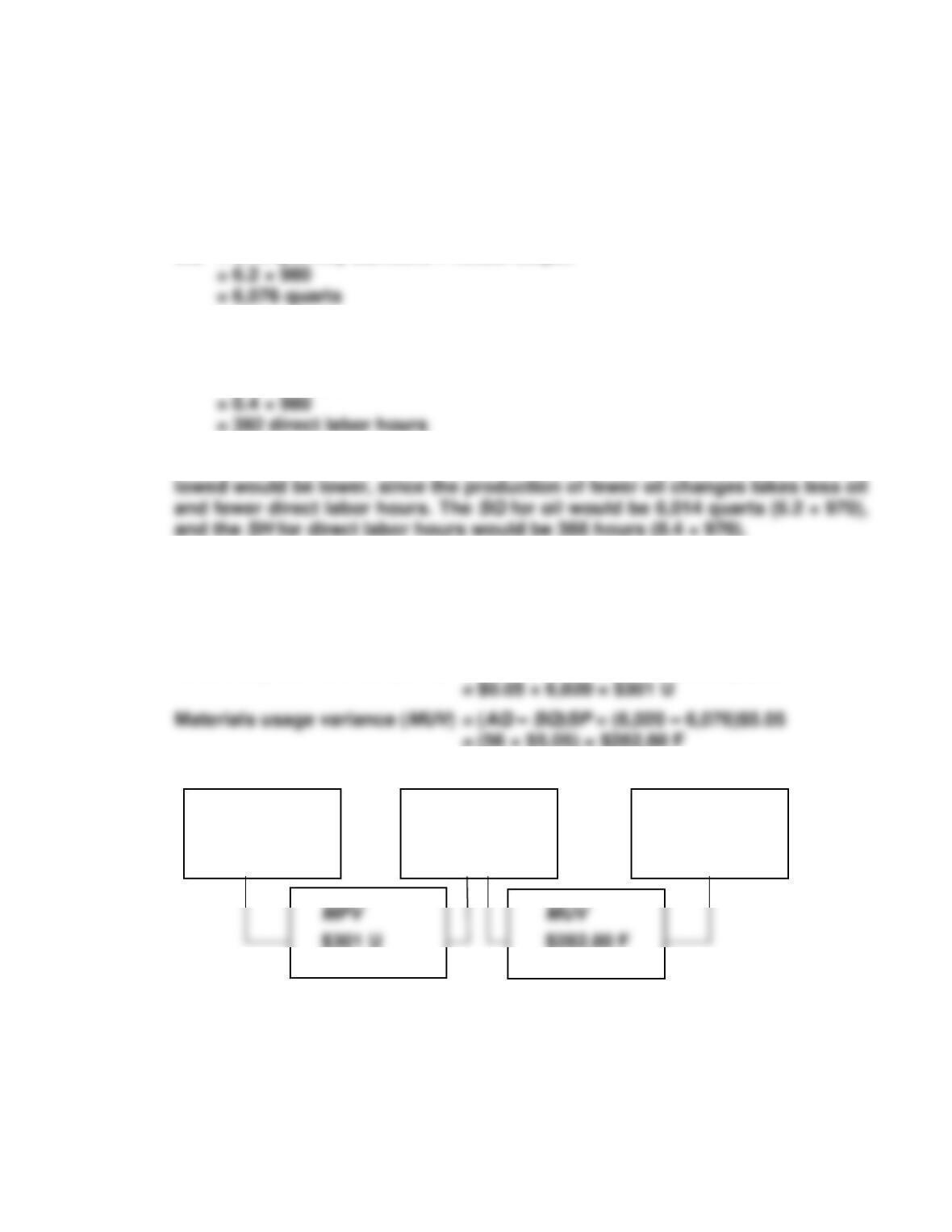
1. Standard quarts of oil allowed:

SQ = Unit quantity standard × Actual output

2. Direct labor hours allowed:

SH = Unit labor standard × Actual output

= (24/60) × 980

3. If 970 oil changes were performed instead of 980, the standard quantities al-

Cornerstone Exercise 9.2

1. Formulas:

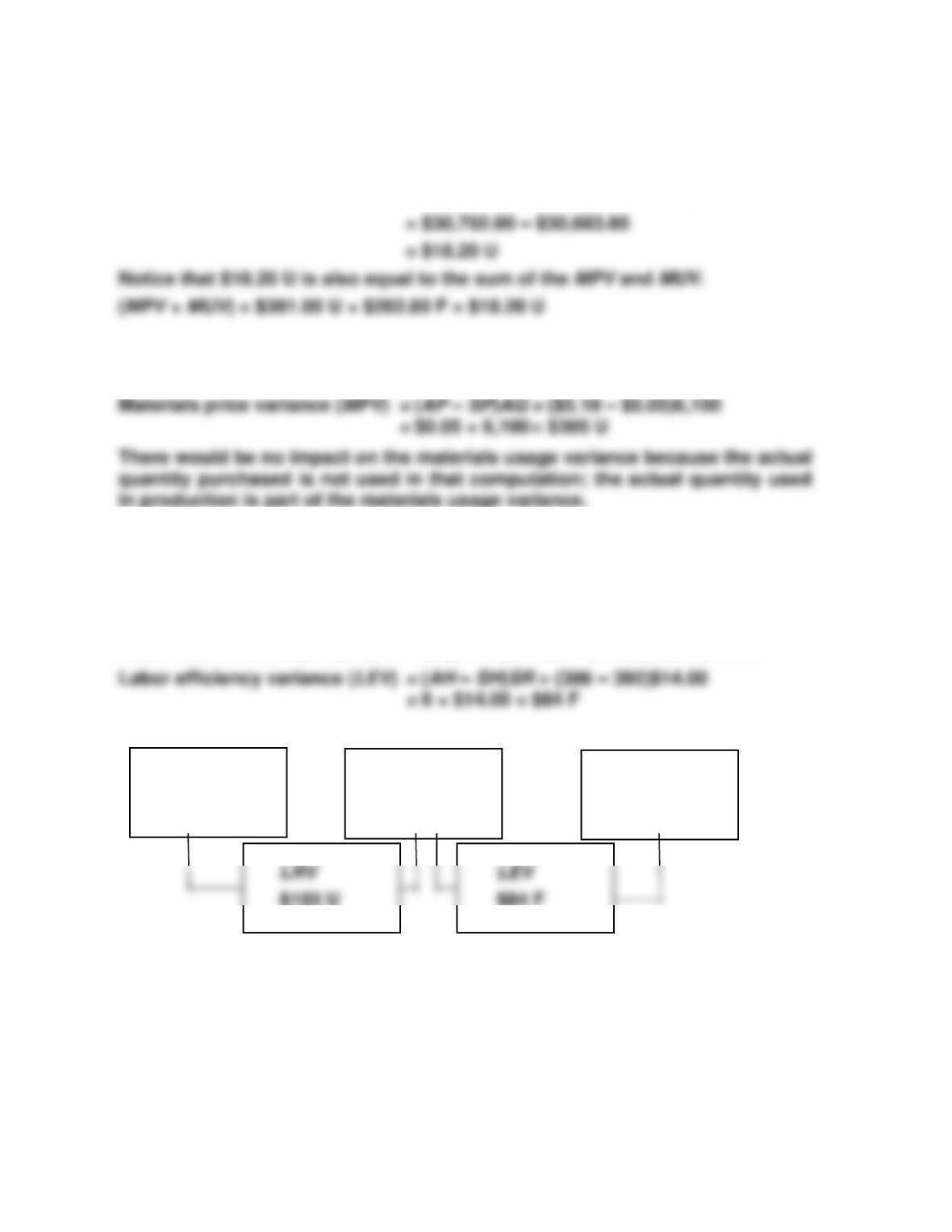
Materials price variance (MPV) = (AP – SP)AQ = ($5.10 – $5.05)6,020

2. AQ × AP AQ × SP SQ × SP

= 6,020 × $5.10 = 6,020 × $5.05 = 6,076 × $5.05

= $30,702.00 = $30,401.00 = $30,683.80

Cornerstone Exercise 9.2 (Concluded)

3. Total direct materials variance = (AP × AQ) × (SP × SQ) = MPV + MUV

= ($5.10 × 6,020) – ($5.05 × 6,076)

4. If the actual quantity purchased was 6,100 quarts, the materials price variance

would be calculated at the time of purchase.

Cornerstone Exercise 9.3

1. Formulas:

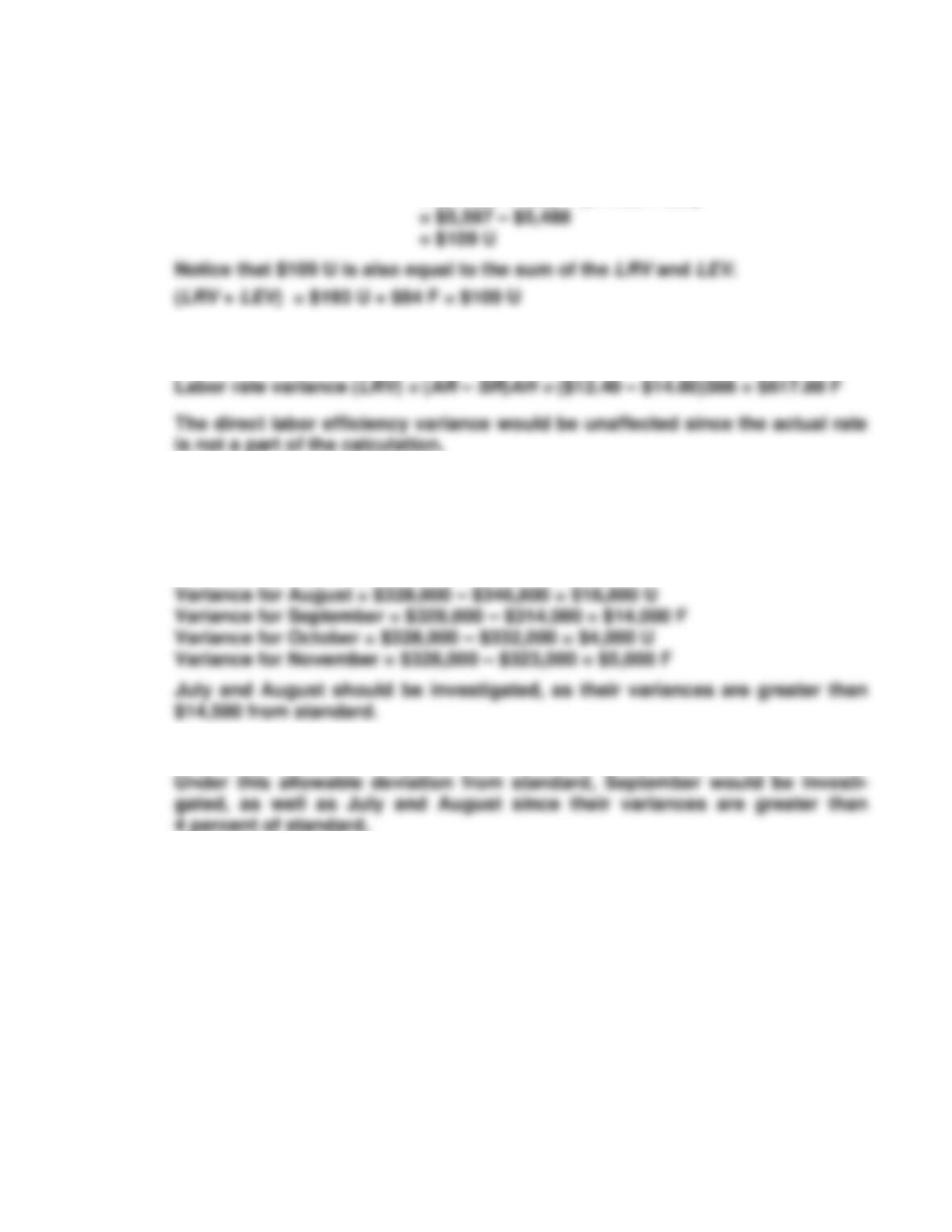
Labor rate variance (LRV) = (AR – SR)AH = ($14.50 – $14.00)386 = $193 U

2. AH × AR AH × SR SH × SR

= 386 × $14.50 = 386 × $14 = 392 × $14

= $5,597 = $5,404 = $5,488

Cornerstone Exercise 9.3 (Concluded)

3. Total direct labor variance = (AR × AH) – (SR × SH) = LRV + LEV

= ($14.50 × 386) – ($14.00 × 392)

4. If the actual direct labor wage rate was $12.40 in June, the direct labor rate

variance would be:

Cornerstone Exercise 9.4

1. Variance for June = $328,000 – $330,500 = $2,500 U

Variance for July = $328,000 – $343,000 = $15,000 U

2. 4% of standard cost = 0.04 × $328,000 = $13,120

Cornerstone Exercise 9.5

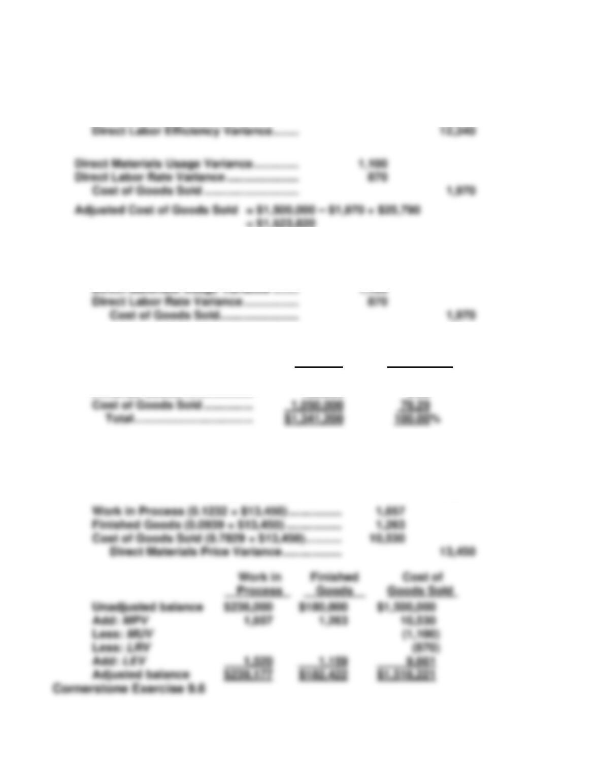
1. Cost of Goods Sold …………………………... 25,790

Direct Materials Price Variance ………. 13,450

2. Immaterial variance account balances are in MUV and LRV. The closing entry

is:

Prime Percentage

Costs of Total

Work in Process ……………….. $165,200 12.32%

Finished Goods ………………… 126,000 9.39

Work in Process (0.1232 × $12,340) ……………. 1,520

Finished Goods (0.0939 × $12,340) …………….. 1,159

Cost of Goods Sold (0.7829 × $12,340) ……….. 9,661

Direct Labor Efficiency Variance …………… 12,340

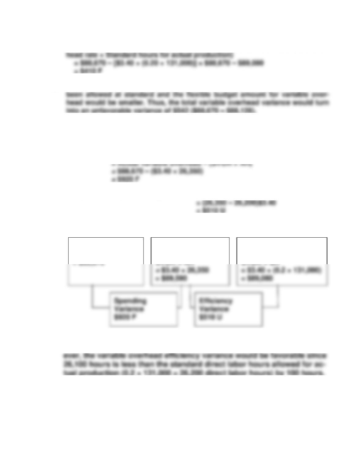
1. Total variable overhead variance = Actual variable overhead – (Variable over-

2. If production had been 129,600 units, fewer direct labor hours would have

Cornerstone Exercise 9.7

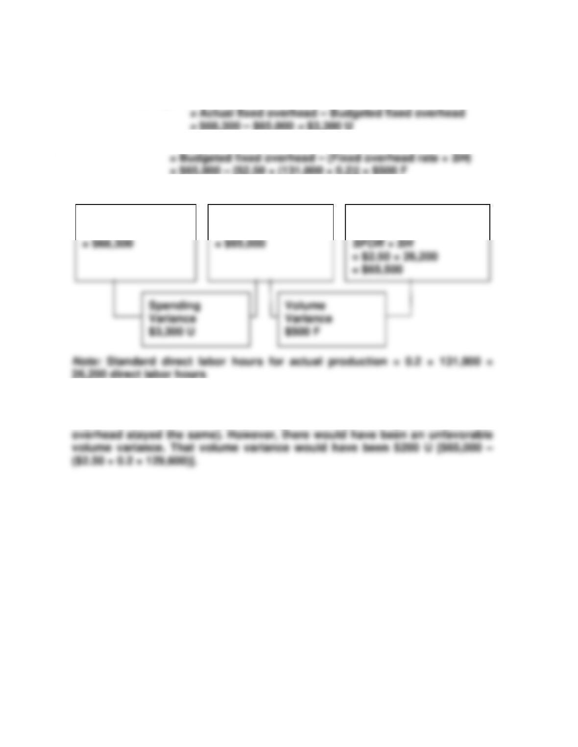
1. Variable overhead spending variance

2. Variable overhead efficiency variance = (AH – SH)SVOR

3.

4. If 26,100 direct labor hours had been worked in February, the variable

overhead spending variance would be smaller, but still favorable. How-

Actual Variable

Overhead

Budgeted Variable

Overhead

Applied Variable

Overhead

Cornerstone Exercise 9.8

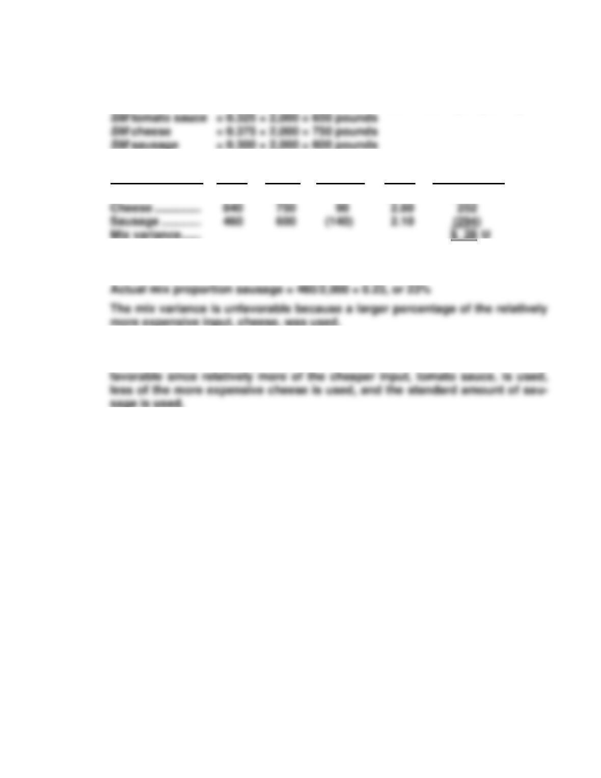
1. Fixed overhead spending variance

2. Volume variance = Budgeted fixed overhead – Applied fixed overhead

3.

4. If 129,600 units had been produced in February, there would have been no

impact on the fixed overhead spending variance (assuming that actual fixed

Actual Fixed

Overhead

Budgeted Fixed

Overhead

Applied Fixed

Overhead

Cornerstone Exercise 9.9

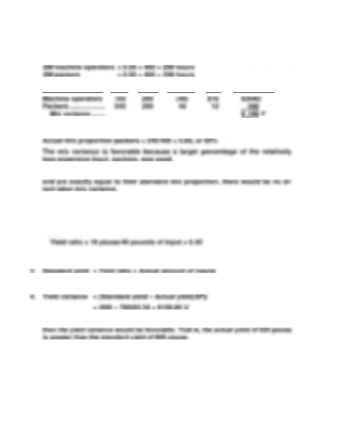
1. SM = Standard mix proportion × Total actual input quantity

2. Direct Material AQ SM AQ – SM SP (AQ – SM)SP

Tomato sauce … 700 650 50 $1.40 $ 70

3. Actual mix proportion tomato sauce = 700/2,000 = 0.35, or 35%

Actual mix proportion cheese = 840/2,000 = 0.42, or 42%

4. Tomato sauce now accounts for 35 percent (700/2,000) of the total, and

cheese accounts for only 35 percent (700/2,000). The mix variance will be

Cornerstone Exercise 9.10

1. SM = Standard mix proportion × Total actual input quantity

2. Direct Labor AQ SM AQ – SM SP (AQ – SM)SP

3. Actual mix proportion machine operators = 160/400 = 0.40, or 40%

4. Since both types of labor account for 50 percent of total direct labor hours,

Cornerstone Exercise 9.11

1. Using the standard mix for 16 pizzas:

2. Standard cost of the yield (SPy) = $85.40/16 pizzas yielded = $5.34 per pizza

= 0.40 × 2,000 pounds = 800 pizzas

5. If the 2,000 pounds of direct materials put into process resulted in 825 pizzas,

EXERCISES

Exercise 9.12

1. Likely coworkers: operating personnel, cost accountants, and engineers. The

operating personnel of each cost center should be involved in setting stand-

ards; they are the primary source for quantity information. The materials

2. The standard prime cost per 10-gallon batch of strawberry jam is as follows:

Strawberries (7.5 qts.a @ $0.80) ………………………. $ 6.00

Other ingredients (10 gals. @ $0.45) ……………….. 4.50

3. Joe has failed to provide decision support information and recommendations

that are accurate, clear, concise, and timely; avoid apparent conflicts of inter-

Exercise 9.13

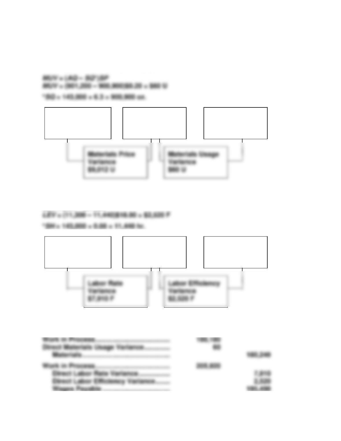
1. SQ = 8.45 lbs. × 280,000 = 2,366,000 pounds

Exercise 9.14

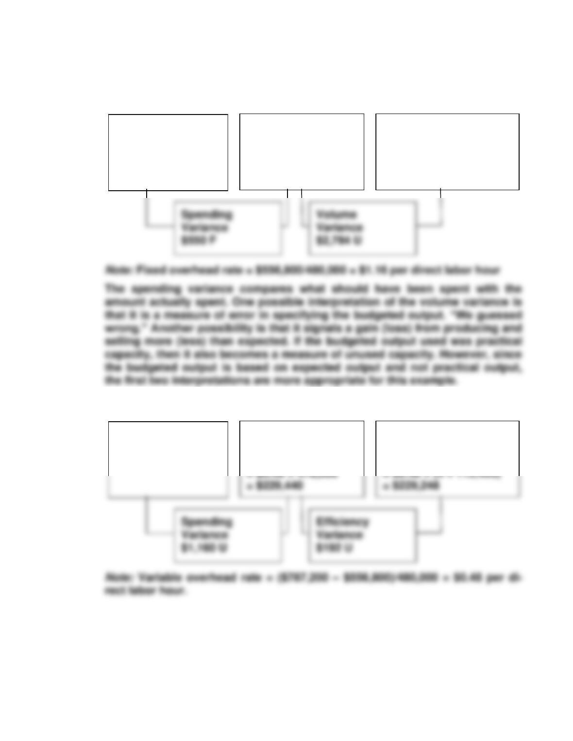
1. MPV = (AP – SP)AQ

MPV = ($0.21 – $0.20)901,200 = $9,012 U

Materials Price

Variance

$9,012 U

Materials Usage

Variance

$60 U

2. LRV = (AR – SR)AH

LRV = ($17.30 – $18.00)11,300 = $7,910 F

LEV = (AH – SH*)SR

Labor Rate

Variance

$7,910 F

Labor Efficiency

Variance

$2,520 F

3. Materials ……………………………………………. 180,240

Direct Materials Price Variance……………. 9,012

Accounts Payable ………………………….. 189,252

AP × AQ

= $0.21 × 901,200

= $189,252

SP × AQ

= $0.20 × 901,200

= $180,240

SP × SQ

= $0.20 × 900,900

= $180,180

AR × AH

= $17.30 × 11,300

= $195,490

SR × AH

= $18 × 11,300

= $203,400

SR × SH

= $18 × 11,440

= $205,920

Exercise 9.15

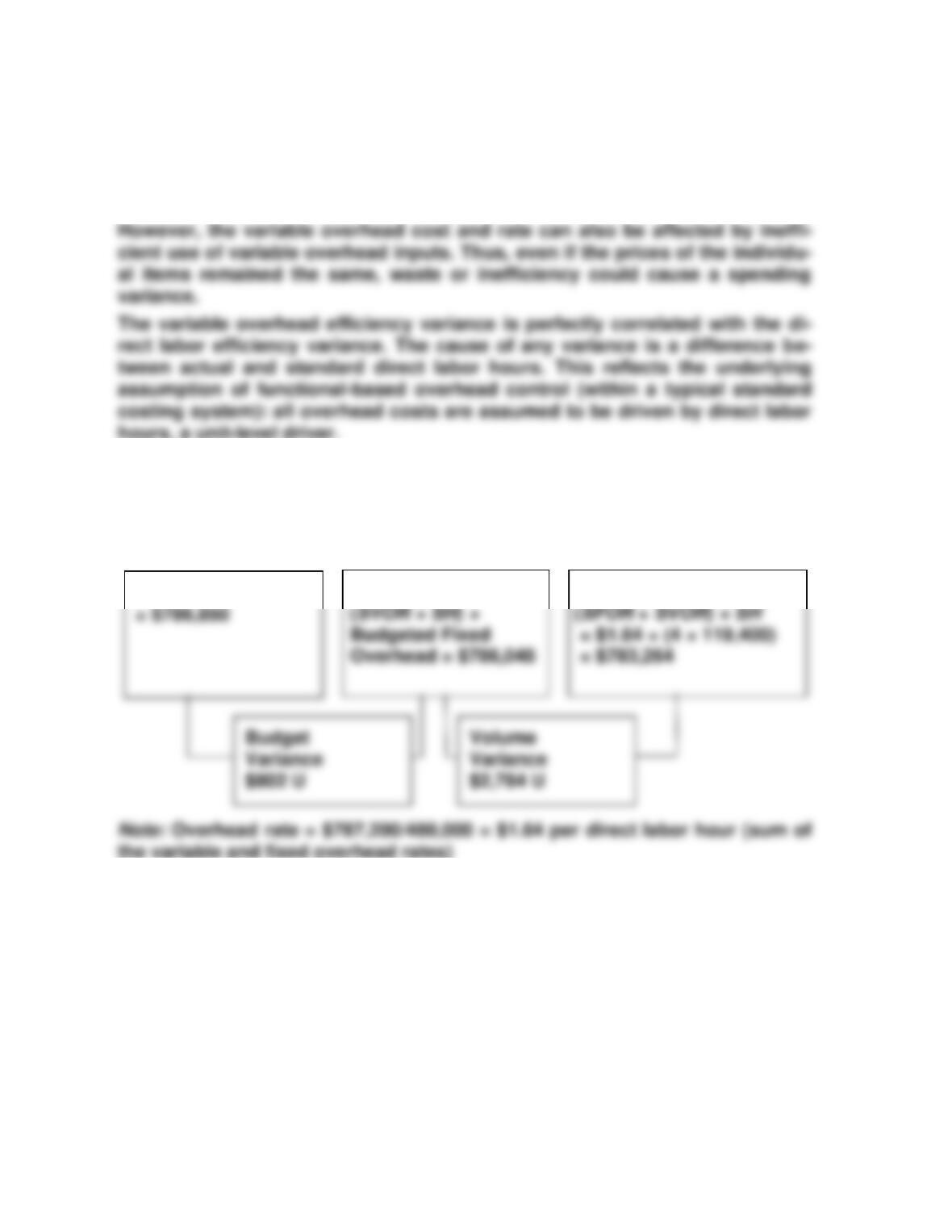
1. Fixed overhead analysis:

2. Variable overhead analysis:

Actual Fixed

Overhead

= $556,250

Budgeted Fixed

Overhead

= $556,800

Applied Fixed

Overhead

SFOR × SH

= $1.16 × (4 × 119,400)

= $554,016

Actual Variable

Overhead

= $230,600

Budgeted Variable

Overhead

SVOR × AH

Applied Variable

Overhead

SVOR × SH

Exercise 9.15 (Concluded)

The variable overhead spending variance can occur because of changes

in the prices of the individual items that make up variable overhead. In this

sense, it is similar to the direct materials and direct labor price variances.

Exercise 9.16

1. Two-variance analysis:

Actual Overhead

Budgeted Overhead

Applied Overhead

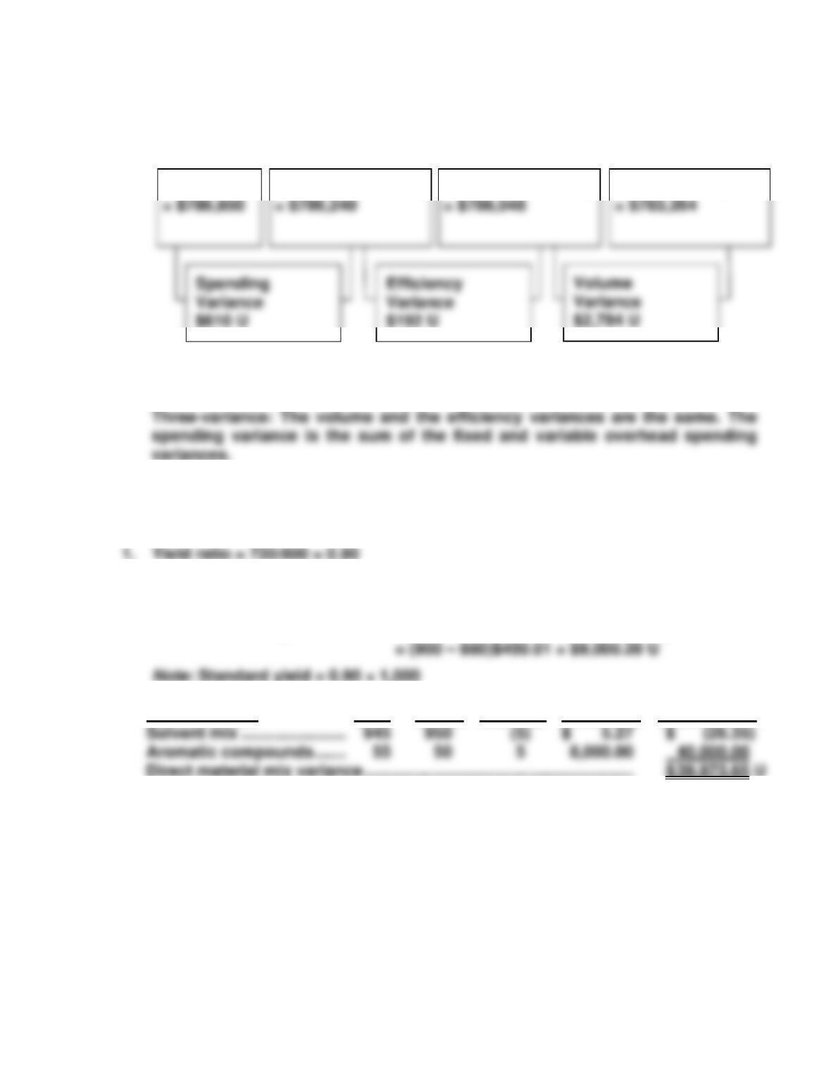
Exercise 9.16 (Concluded)

2. Three-variance analysis (BFOH = Budgeted fixed overhead; OH = Overhead):

3. Two-variance: The volume variance is the same. The budgeted variance is the

sum of the fixed and variable spending variances and the efficiency variance.

Exercise 9.17

2. SPy = $324,005.20/720 = $450.01

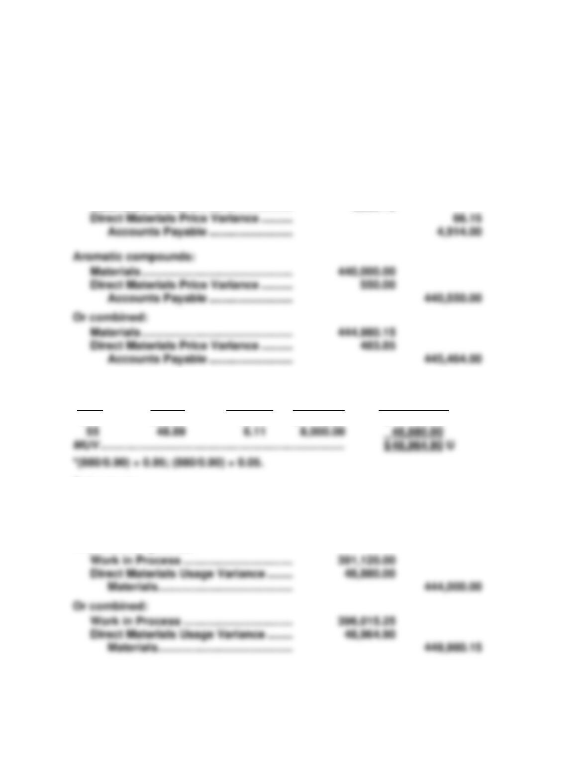
3. Direct materials yield variance = (Standard yield – Actual yield)SPy

4. Direct Material AQ SM AQ – SM SP (AQ – SM)SP

Actual OH

BFOH + (SVOR × AH)

BFOH + (SVOR × SH)

(SFOH + SVOR) × SH

Exercise 9.18

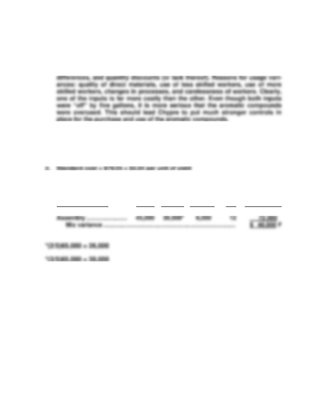
1. MPV = (AP – SP)AQ

Solvent mix:

MPV = ($5.20 – $5.27)945 = $66.15 F

Aromatic compounds:

MPV = ($8,010 – $8,000)55 = $550.00 U

Solvent mix:

Materials ……………………………………….. 4,980.15

2. Materials usage variance:

AQ SQ* AQ – SQ SP (AQ – SQ)SP

945 928.89 16.11 $ 5.27 $ 84.90

Solvent mix:

Work in Process ……………………………. 4,895.25

Direct Materials Usage Variance …….. 84.90

Materials…………………………………… 4,980.15

Aromatic compounds:

Exercise 9.18 (Concluded)

3. The direct materials price and usage variances are both favorable and unfa-

vorable. Reasons for price variances: random market fluctuation of the input

prices, permanent changes in the input prices, changes in suppliers, quality

Exercise 9.19

1. Yield ratio = 25 units/5 hours = 5

3. Direct labor yield variance = (Standard yield – Actual yield)SPy

= (325,000 – 320,000)$3.04 = $15,200 U

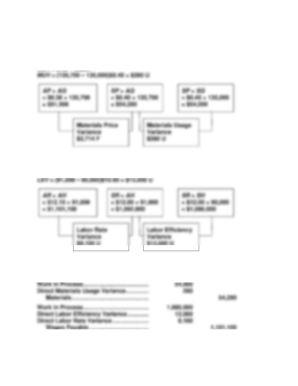
4. Direct Labor Type AH SM AH – SM SP (AH – SM)SP

Fabricating …………………. 20,000 26,000* (6,000) $ 20 $(120,000)

Exercise 9.20

1. MPV = (AP – SP)AQ

MPV = ($0.38 – $0.40)135,700 = $2,714 F

2. LRV = (AR – SR)AH

LRV = ($12.10 – $12.00)91,000 = $9,100 U

LEV = (AH – SH)SR

3. Materials ……………………………………………. 54,280

Direct Materials Price Variance ………. 2,714

Accounts Payable ………………………….. 51,566

Exercise 9.20 (Concluded)

Exercise 9.21

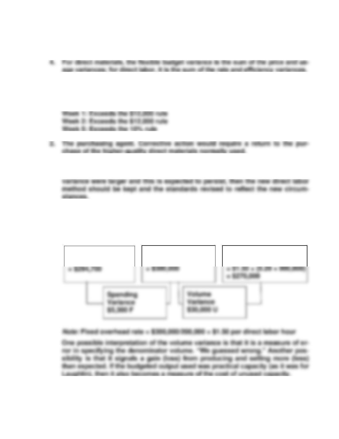
1. Cases needing investigation:

3. Production engineering is responsible. If the relationship is expected to per-

sist, then the new direct labor method should be abandoned. If the favorable

Exercise 9.22

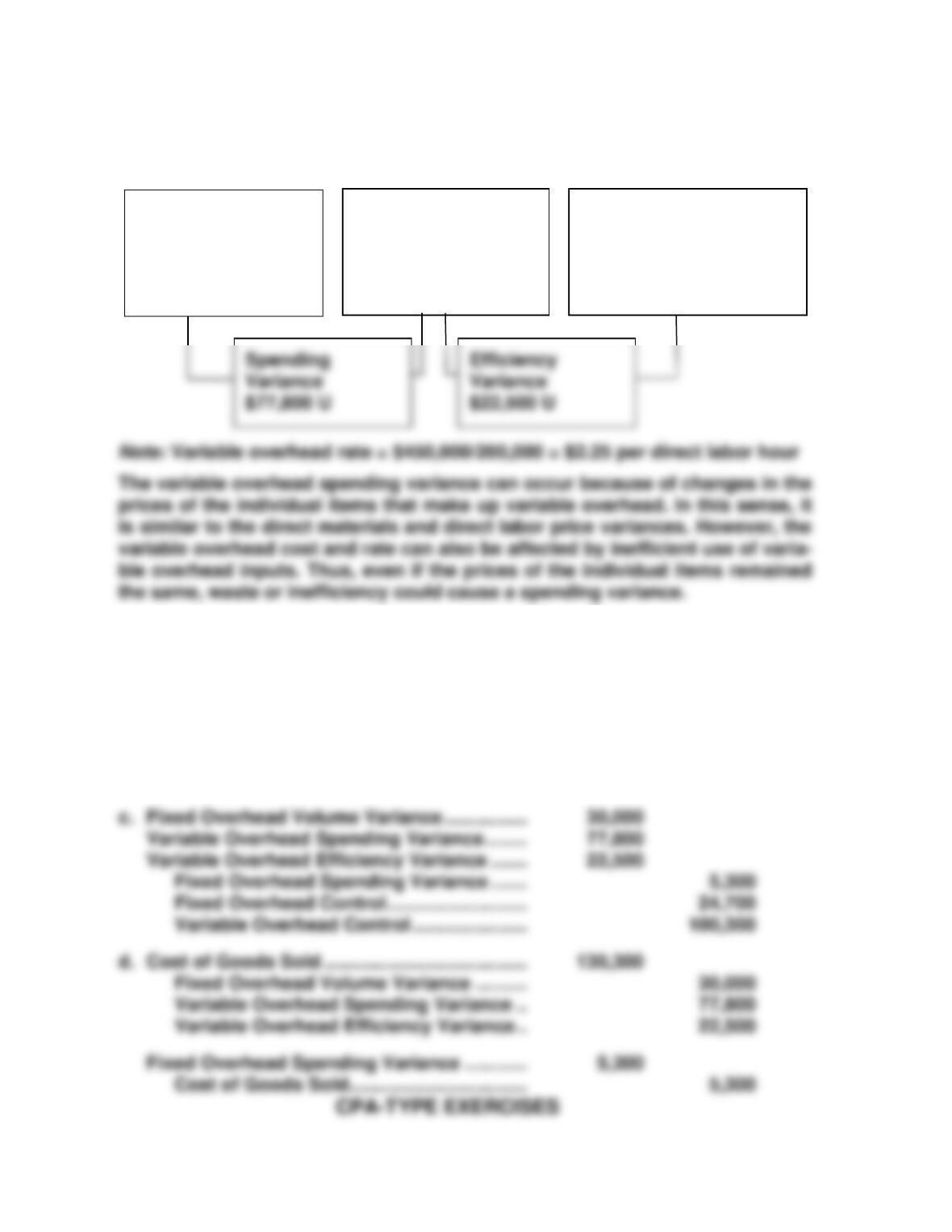
1. Fixed overhead analysis:

Actual Fixed

Overhead

Budgeted Fixed

Overhead

Applied Fixed Overhead

SFOR × SH

Exercise 9.22 (Concluded)

2. Variable overhead analysis:

3. Journal entries:

a. Work in Process …………………………………….. 675,000

Variable Overhead Control …………………. 405,000

Fixed Overhead Control……………………… 270,000

b. Variable Overhead Control ……………………… 505,300

Fixed Overhead Control ………………………….. 294,700

Miscellaneous Accounts ……………………. 800,000

Actual Variable

Overhead

= $505,300

Budgeted Variable

Overhead

SVOR × AH

= $2.25 × 190,000

= $427,500

Applied Variable

Overhead

SVOR × SH

= $2.25 × 0.20 × 900,000

= $405,000