PROBLEM 8.3 (Continued)
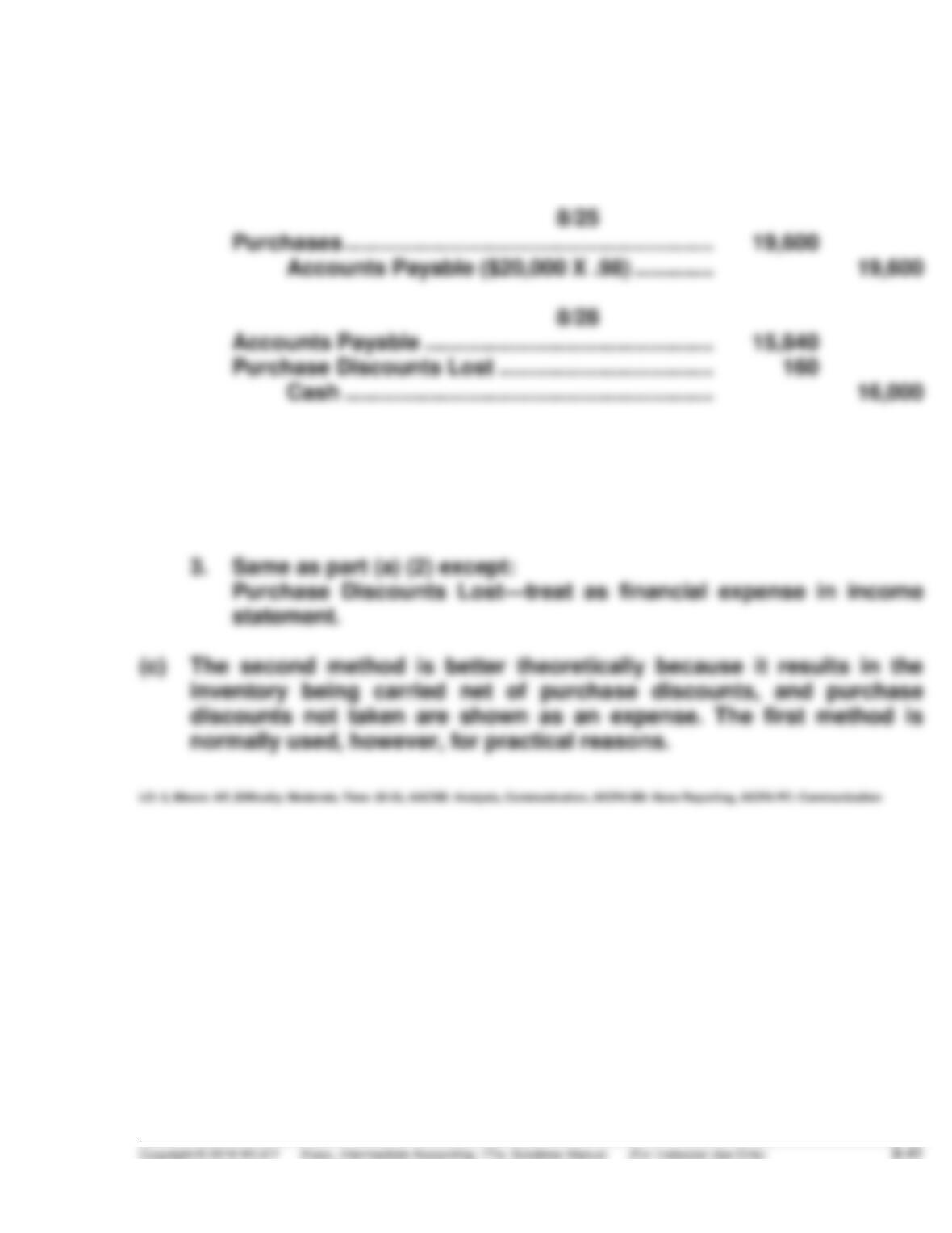
8/15
Purchases ………………………………………………………
15,840
Accounts Payable ($16,000 X .99) …………….
15,840
8/25
Purchases ………………………………………………………
19,600
Accounts Payable ($20,000 X .98) …………….
19,600
Accounts Payable …………………………………………..
15,840
Purchase Discounts Lost ………………………………..
Cash ………………………………………………………
16,000
2.
8/31
Purchase Discounts Lost ………………………………..
216
Accounts Payable
(.02 X [$12,000 – $1,200]) ………………………
216
3.
Same as part (a) (2) except:
PROBLEM 8.4
(a)
Purchases
Total Units
Sales
Total Units
April 1 (balance on hand)
100
April 5
300
April 4
400
April 12
200
April 11
300
April 27
800
April 18
200
April 28
April 30
Total units
Total units sold
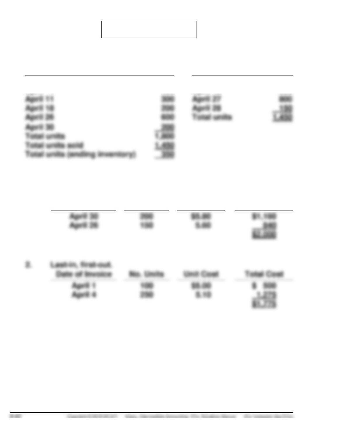
Assuming costs are not computed for each withdrawal:
1. First-in, first-out.
Date of Invoice
No. Units
Unit Cost
Total Cost
Date of Invoice
No. Units
Unit Cost
Total Cost
PROBLEM 8.4 (Continued)
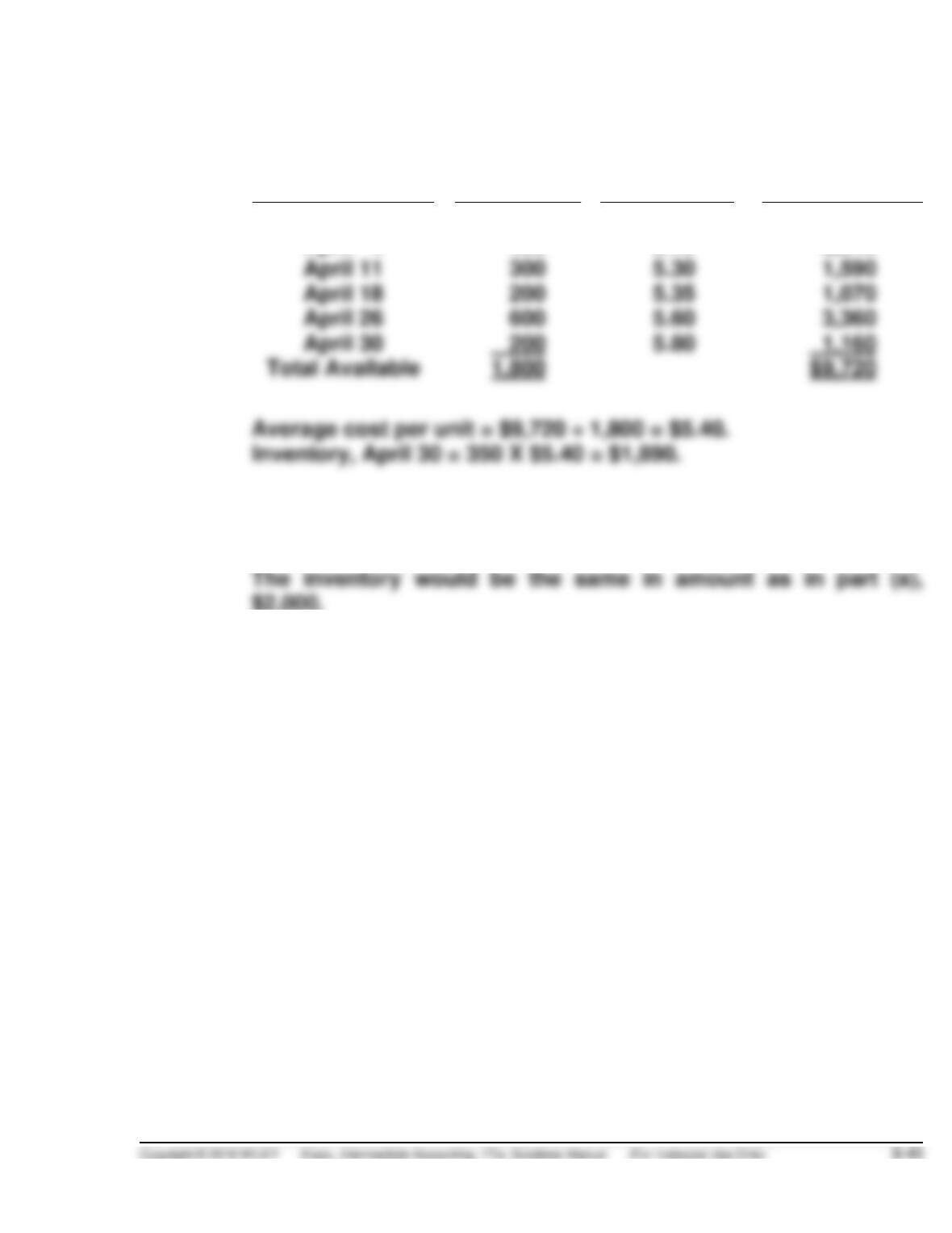
3. Average-cost.
Cost of Part X available.
Date of Invoice
No. Units
Unit Cost
Total Cost
April 1
100
$5.00
$ 500
April 4
400
5.10
2,040
April 26
600
5.60
3,360
(b) Assuming costs are computed for each withdrawal:
1. First-in, first out.
PROBLEM 8.4 (Continued)
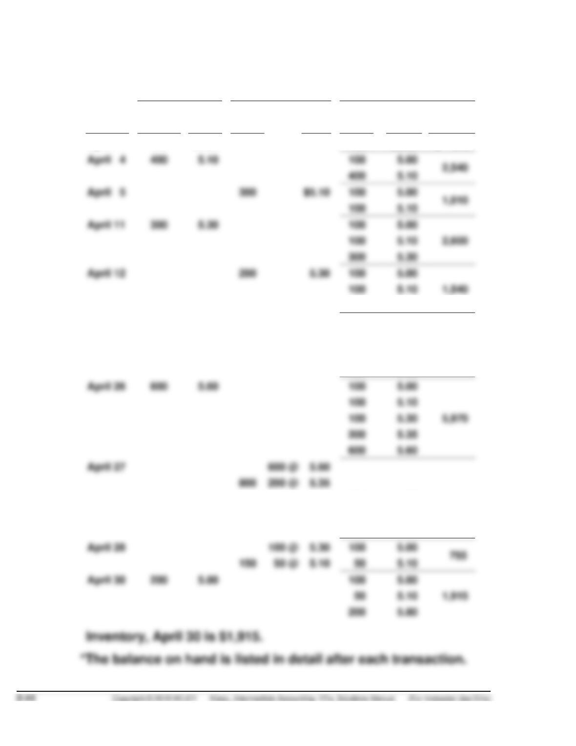
2. Last-in, first-out.
Purchased
Sold
Balance*
Date
No. of
units
Unit
cost
No. of
units
Unit
cost
No. of
units
Unit
cost
Amount
April 1
100
$5.00
100
$5.00
$ 500
April 4
100
5.00
2,540
400
5.10
April 5
300
$5.10
100
5.00
100
5.10
100
5.10
300
5.30
April 12
200
100
5.00
100
5.10
100
5.30
April 18
200
5.35
100
5.00
100
5.10
2,610
100
5.30
200
5.35
April 26
100
5.00
100
5.10
100
5.30
200
5.35
600
5.60
April 27
800
100
5.00
1,540
100
5.10
100
5.30
April 28
100
5.00
150
5.10
April 30
200
100
5.00
5.10
200
5.80
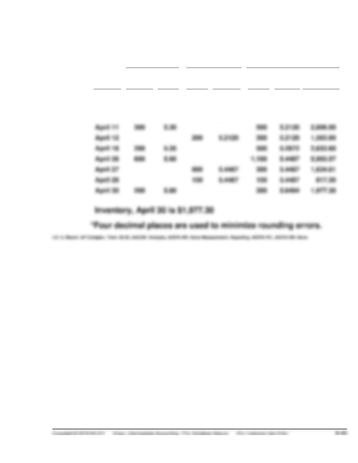
PROBLEM 8.4 (Continued)
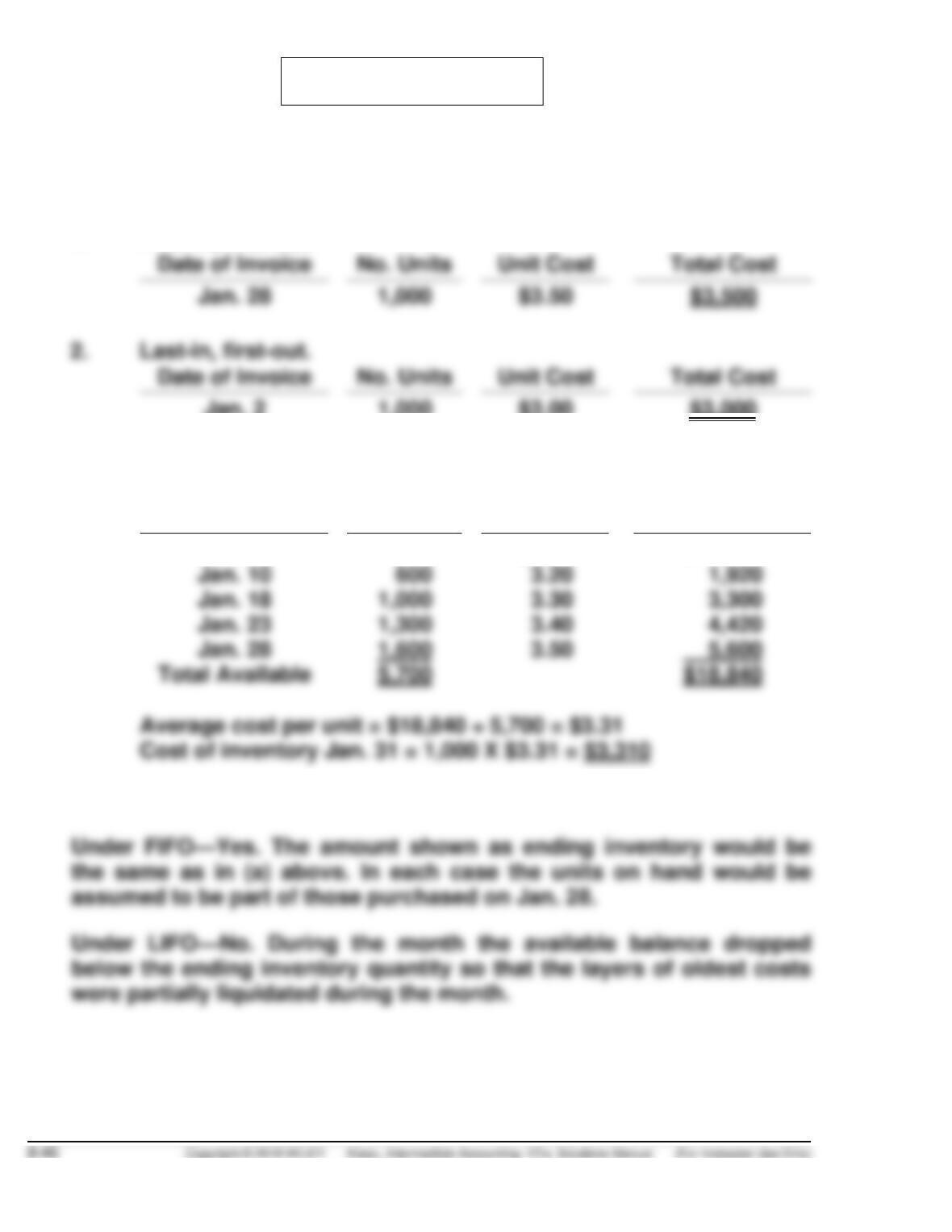
3. Average-cost.
Purchased
Sold
Balance
Date
No. of
units
Unit
cost
No. of
units
Unit
cost
No. of
units
Unit
cost*
Amount
April 1
100
$5.00
100
$5.0000
$ 500.00
April 4
400
5.10
500
5.0800
2,540.00
April 5
300
$5.0800
200
5.0800
1,016.00
April 11
300
5.30
500
5.2120
2,606.00
April 12
200
5.2120
300
5.2120
1,563.60
April 18
200
5.35
500
5.2672
2,633.60
April 26
600
5.60
1,100
5.4487
5,993.57
April 27
800
5.4487
300
5.4487
1,634.61
April 28
150
5.4487
150
5.4487
817.30
April 30
200
5.80
350
5.6494
1,977.30
PROBLEM 8.5
(a) Assuming costs are not computed for each withdrawal (units received,
5,700, minus units issued, 4,700, equals ending inventory of 1,000 units):
1. First-in, first-out.
Date of Invoice
No. Units
Unit Cost
Total Cost
$3.50
Date of Invoice
No. Units
Unit Cost
Total Cost
Jan. 2
1,000
$3.00
$3,000
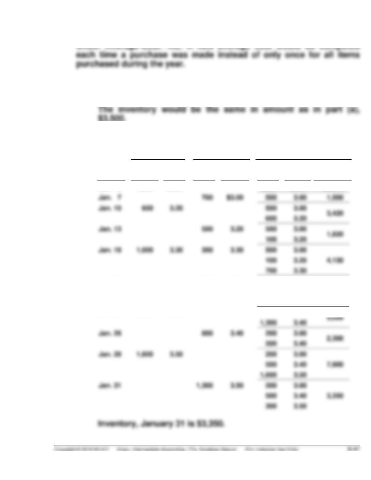
3. Average-cost.
Cost of goods available:
Date of Invoice
No. Units
Unit Cost
Total Cost
Jan. 2
1,200
$3.00
$ 3,600
Jan. 23
1,300
4,420
(b) Assuming costs are computed at the time of each withdrawal:
PROBLEM 8.5 (Continued)
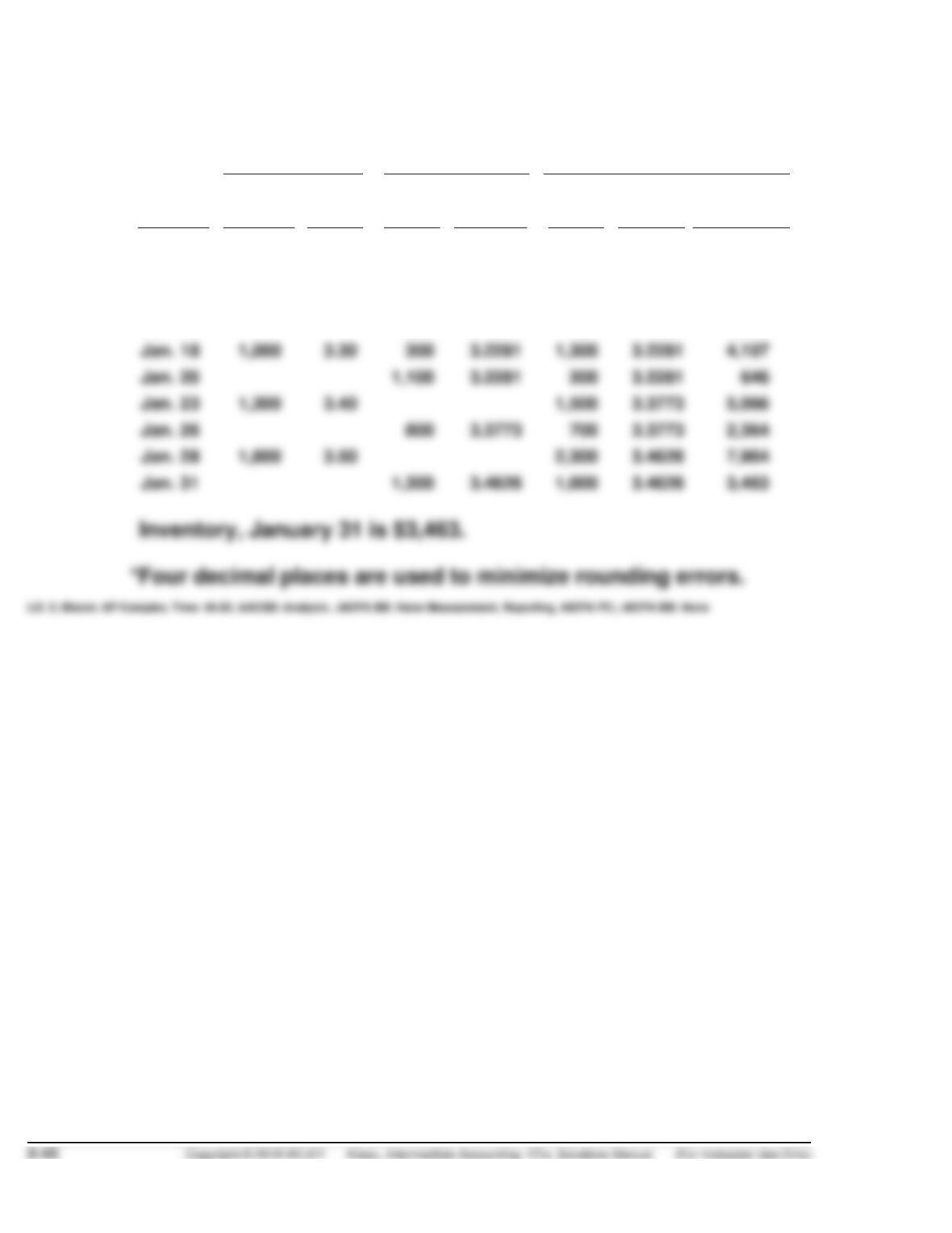
The calculations to determine the inventory on this basis are given below.
1. First-in, first-out.
2. Last-in, first-out.
Received
Issued
Balance
Date
No. of
units
Unit
cost
No. of
units
Unit
cost
No. of
units
Unit
cost*
Amount
Jan. 2
1,200
$3.00
1,200
$3.00
$3,600
Jan. 7
700
$3.00
500
3.00
1,500
Jan. 10
600
3.20
500
3.00
600
Jan. 13
500
3.20
500
3.00
100
3.20
Jan. 18
1,000
3.30
300
3.30
500
3.00
100
4,130
700
3.30
Jan. 20
700
3.30
100
3.20
300
3.00
200
3.00
600
Jan. 23
1,300
3.40
200
3.00
1,300
3.40
Jan. 26
800
3.40
200
500
3.40
Jan. 28
1,600
3.50
200
3.00
500
3.40
7,900
1,600
Jan. 31
1,300
3.50
200
3.00
500
3.40
3,350
PROBLEM 8.5 (Continued)
3. Average-cost.
Received
Issued
Balance
Date
No. of
units
Unit
cost
No. of
units
Unit
cost
No. of
units
Unit
cost*
Amount
Jan. 2
1,200
$3.00
1,200
$3.0000
$3,600
Jan. 7
700
$3.0000
500
3.0000
1,500
Jan. 10
600
3.20
1,100
3.1091
3,420
Jan. 13
500
3.1091
600
3.1091
1,865
Jan. 18
300
1,300
3.2281
4,197
1,100
3.2281
200
3.2281
646
Jan. 23
1,300
3.40
1,500
3.3773
5,066
Jan. 26
800
700
3.3773
2,364
Jan. 28
1,600
3.50
2,300
3.4626
7,964
Jan. 31
1,300
3.4626
1,000
3.4626
3,463
PROBLEM 8.6
(a)
Beginning inventory …………………
1,000
Purchases (2,000 + 3,000) ………….
5,000
Units available for sale ……………..
6,000
Sales (2,500 + 2,200) …………………
Goods on hand …………………………
Periodic FIFO
1,000 X $12 =
2,000 X $18 =
1,700 X $23 =
4,700
$87,100
(b)
Perpetual FIFO
Same as periodic:
$87,100
(c)
Periodic LIFO
3,000 X $23 =
1,700 X $18 =
4,700
$99,600
(d)
Perpetual LIFO
Date
Purchased
Sold
Balance
1/1
1,000 X $12
=
$12,000
2,000 X $18 = $36,000
1,000 X $12
2,000 X $18
2/20
2,000 X $18
500 X $12
500 X $12
=
$ 6,000
4/2
3,000 X $23 = $69,000
500 X $12
3,000 X $23
11/4
2,200 X $23
=
$50,600
500 X $12
PROBLEM 8.6 (Continued)
(e)
Periodic weighted-average
1,000 X $12 =
2,000 X $18 =
3,000 X $23 =
$91,650
(f)
Perpetual moving average
Date
Purchased
Sold
Balance
1/1
1,000 X $12 =
$12,000
2/4
2,000 X $18 = $36,000
2/20
2,500 X $16 =
$40,000
500 X $16 =
8,000
4/2
3,000 X $23 = $69,000
3,500 X $22a =
11/4
2,200 X $22 =
$88,400
3,000 X $23 = 69,000
PROBLEM 8.7
The accounts in the 2021 financial statements which would be affected by
a change to LIFO and the new amount for each of the accounts are as
follows:
Account
New amount
for 2021
(1)
Cash
$176,400
(2)
Inventory
(3)
Retained earnings
(4)
Cost of goods sold
(5)
Income taxes
The calculations for both 2020 and 2021 to support the conversion to LIFO
are presented below.
Income for the Years Ended
12/31/20
12/31/21
Sales revenue
$900,000
$1,350,000
Less: Cost of goods sold
792,000
Other expenses
304,000
Income before taxes
254,000
Cost of Goods Sold and
Ending Inventory for the Years Ended
12/31/20
12/31/21
Beginning inventory
( 40,000 X $3.00)
$120,000
( 40,000 X $3.00)
$120,000
Purchases
(150,000 X $3.50)
(180,000 X $4.40)
792,000
Cost of goods available
912,000
Ending inventory
( 40,000 X $3.00)
( 40,000 X $3.00)
Cost of goods sold
Determination of Cash at
12/31/20
12/31/21
Income taxes under FIFO
$ 76,000
$116,000
Income taxes as calculated under LIFO
68,000
101,600
Increase in cash
8,000
14,400
difference
8,000
Total increase in cash
8,000
22,400
PROBLEM 8.7 (Continued)
Determination of Retained Earnings at
12/31/20
12/31/21
Net income under FIFO
$114,000
$174,000
Net income under LIFO
(102,000)
(152,400)
Reduction in retained earnings
12,000
21,600
2020 reduction
12,000
Total reduction in retained earnings
12,000
33,600
Retained earnings under FIFO
LO: 3, Bloom: AP, Difficulty: Moderate, Time: 30–40, AACSB: Analysis, AICPA BB: None Reporting, AICPA PC:, AICPA BB: None
PROBLEM 8.8
(a)
1.
Ending inventory in units
Portable
6,000 + 15,000 – 14,000 =
7,000
Midsize
8,000 + 20,000 – 24,000 =
Flat-screen
3,000 + 10,000 – 6,000 =
2.
Ending inventory at current cost
Portable
7,000 X $110 =
$ 770,000
Midsize
4,000 X $300 =
Flat-screen
7,000 X $500 =
3.
Ending inventory at base-year cost
Portable
7,000 X $100 =
$ 700,000
Midsize
4,000 X $250 =
Flat-screen
7,000 X $400 =
4.
Price index
$5,470,000 ÷ $4,500,000 = 1.2156
5.
Ending inventory
$3,800,000 X 1.0000 =
$3,800,000
700,000* X 1.2156 =
850,920
*($4,500,000 – $3,800,000 = $700,000)
6.
Cost of goods sold
Beginning inventory ………………………………………….
$ 3,800,000
Purchases
Cost of goods available …………………………………….
Ending inventory ………………………………………………
PROBLEM 8.8 (Continued)
7.
Gross profit
Sales revenue
(6,000 X $600)] …………………………………………………….
$15,420,000
Cost of goods sold …………………………………………………
(b)
1.
Ending inventory at current cost restated to base cost
Portable
$ 770,000 ÷ 1.10a =
$ 700,000
a. $110 ÷ $100
b. $300 ÷ $250
c. $500 ÷ $400
2.
Ending inventory
Portable
$ 600,000 X 1.00 =
$ 600,000
100,000 X 1.10 =
Midsize
Flat-screen
2,000,000
3.
Cost of good sold
Cost of good available …………………………………………
$16,450,000
Ending inventory …………………………..…………………….
Cost of goods sold …………………………………………
$11,540,000
4.
Gross profit
Sales revenue ……………………………………………………..
$15,420,000
Cost of goods sold ………………………………………………
PROBLEM 8.9
(a) BONANZA WHOLESALERS INC.
Computation of Internal Conversion Price Index
for Inventory Pool No. 1 Double Extension Method
Current inventory at
current-year cost
2020
2021
Product A
17,000 X $36 =
$612,000
13,000 X $40 =
$520,000
base cost
17,000 X $30 =
Product B
10,000 X $25 =
Conversion price index $846,000 ÷ $735,000 = 1.15 $840,000 ÷ $640,000 = 1.31
(b) BONANZA WHOLESALERS INC.
Computation of Inventory Amounts
Under Dollar-Value LIFO Method for Inventory Pool No. 1
at December 31, 2020 and 2021
Current
Inventory at
base cost
Conversion
price index
Inventory at
LIFO cost
December 31, 2020
Base inventory
$525,000
1.00
$525,000
(a)
$525,000
2020 layer (remaining)
1.15
(a)
PROBLEM 8.10
Base-Year
Cost
Index %
Dollar-Value
LIFO
December 31, 2019
January 1, 2019, base
$45,000
100
$45,000
December 31, 2019, layer
11,000
12,320
December 31, 2020
January 1, 2019, base
$45,000
100
December 31, 2019, layer
11,000
112
12,320
December 31, 2020, layer
December 31, 2021
January 1, 2019, base
$45,000
100
$45,000
December 31, 2019, layer
11,000
112
12,320
December 31, 2020, layer
12,400
128
15,872
December 31, 2021, layer
1,600
2,080
*$62,700 ÷ $56,000
***$90,800 ÷ $70,000
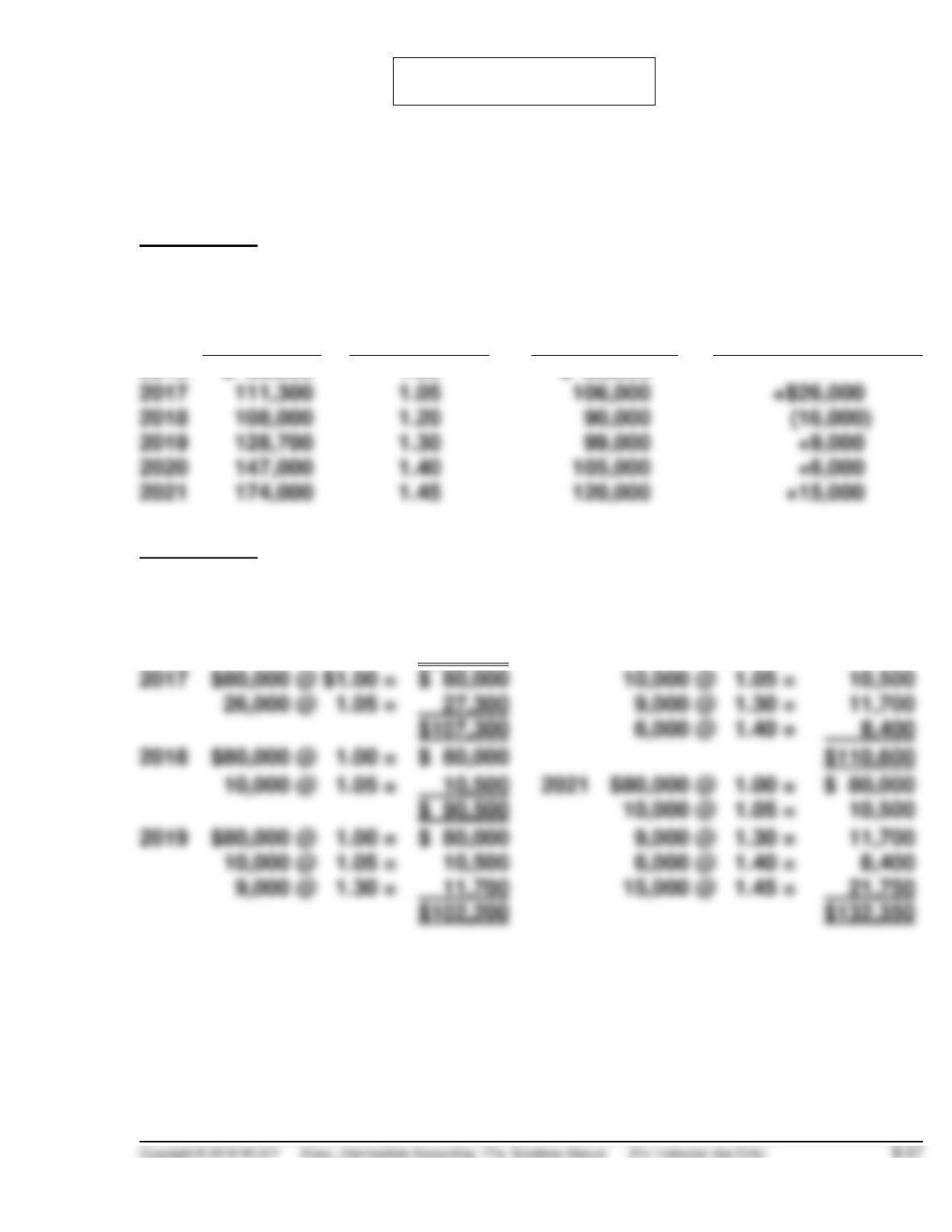
PROBLEM 8.11
(a)
Schedule A
A
B
C
D
Current $
Price Index
Base-Year $
Change from
Prior Year
2016
$ 80,000
1.00
$ 80,000
—
2017
1.05
2019
1.30
99,000
2020
1.40
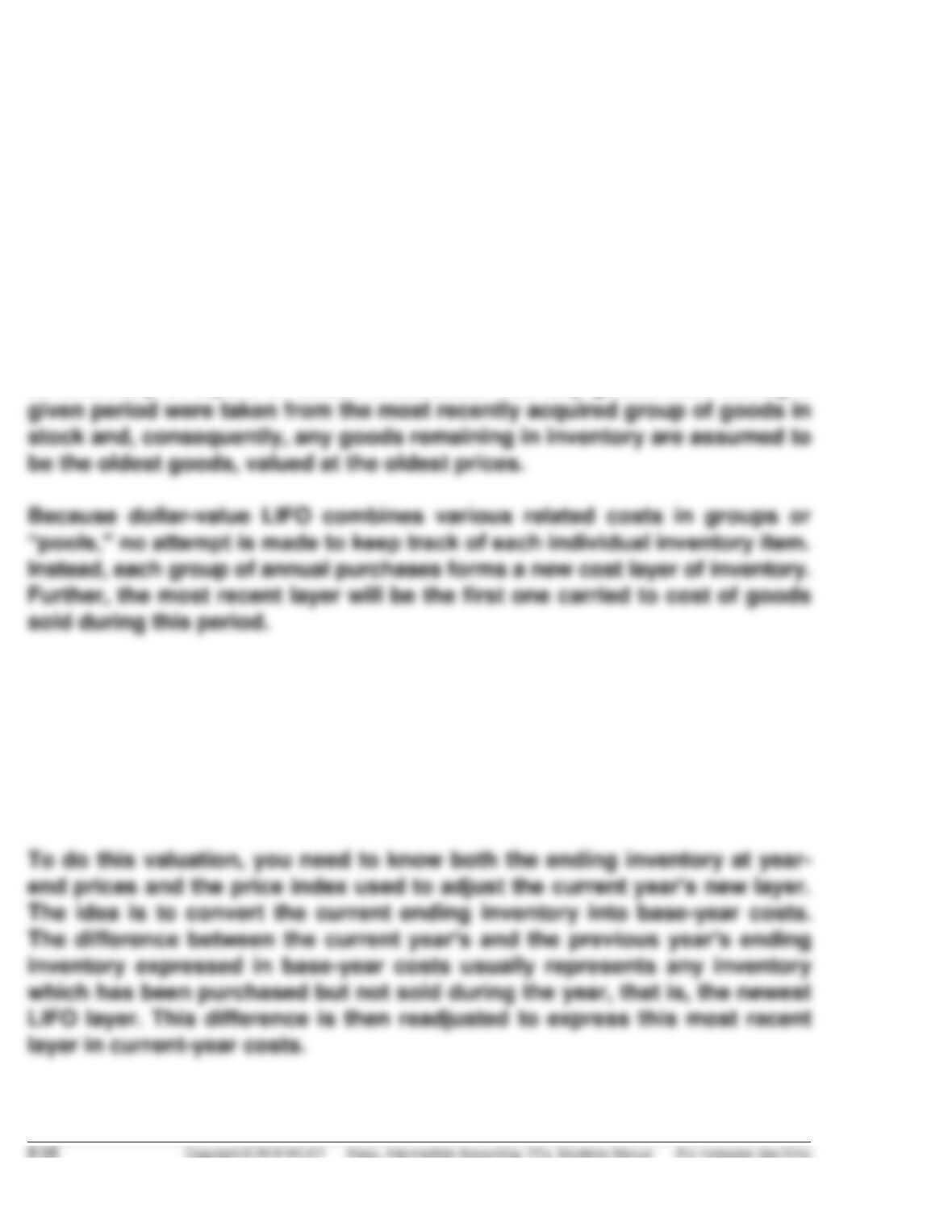
Schedule B
Ending Inventory-Dollar-Value LIFO:
2016
$ 80,000
2020
$80,000 @ $1.00 =
$ 80,000
27,300
9,000 @ 1.30 =
10,500
2021
$80,000 @ 1.00 =
$ 80,000
6,000 @ 1.40 =
9,000 @ 1.30 =
11,700
21,750
PROBLEM 8.11 (Continued)
(b)
To: Richardson Company
From: Accounting Student
Subject: Dollar-Value LIFO Pool Accounting
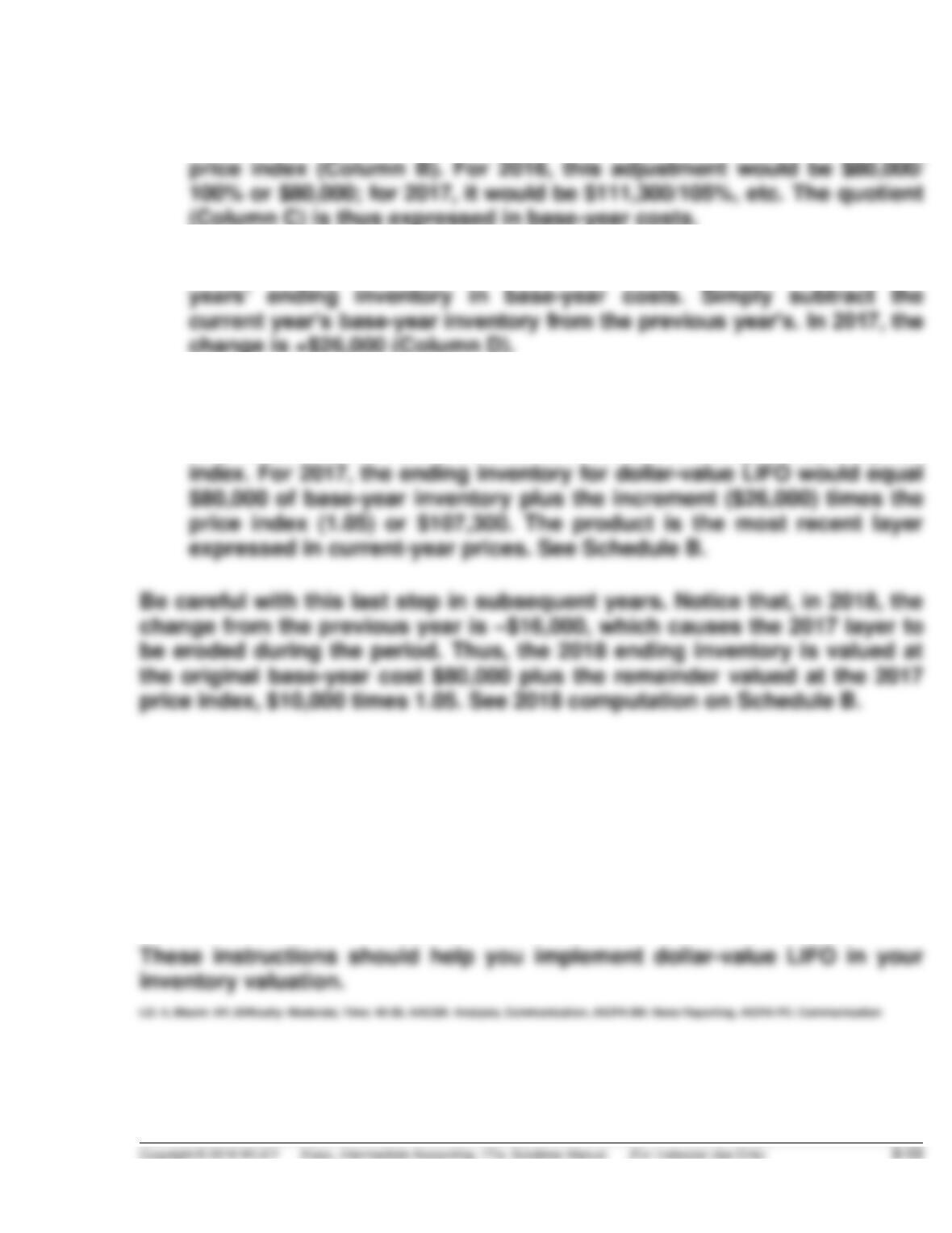
Dollar-value LIFO is an inventory method which values groups or “pools”
of inventory in layers of costs. It assumes that any goods sold during a
However, inflation distorts any cost of purchases made in subsequent years.
To counteract the effect of inflation, this method measures the incremental
change in each year’s ending inventory in terms of the first year’s (base
year’s) costs. This is done by adjusting subsequent cost layers, through
the use of a price index, to the base year’s inventory costs. Only after this
adjustment can the new layer be valued at current-year prices.
PROBLEM 8.11 (Continued)
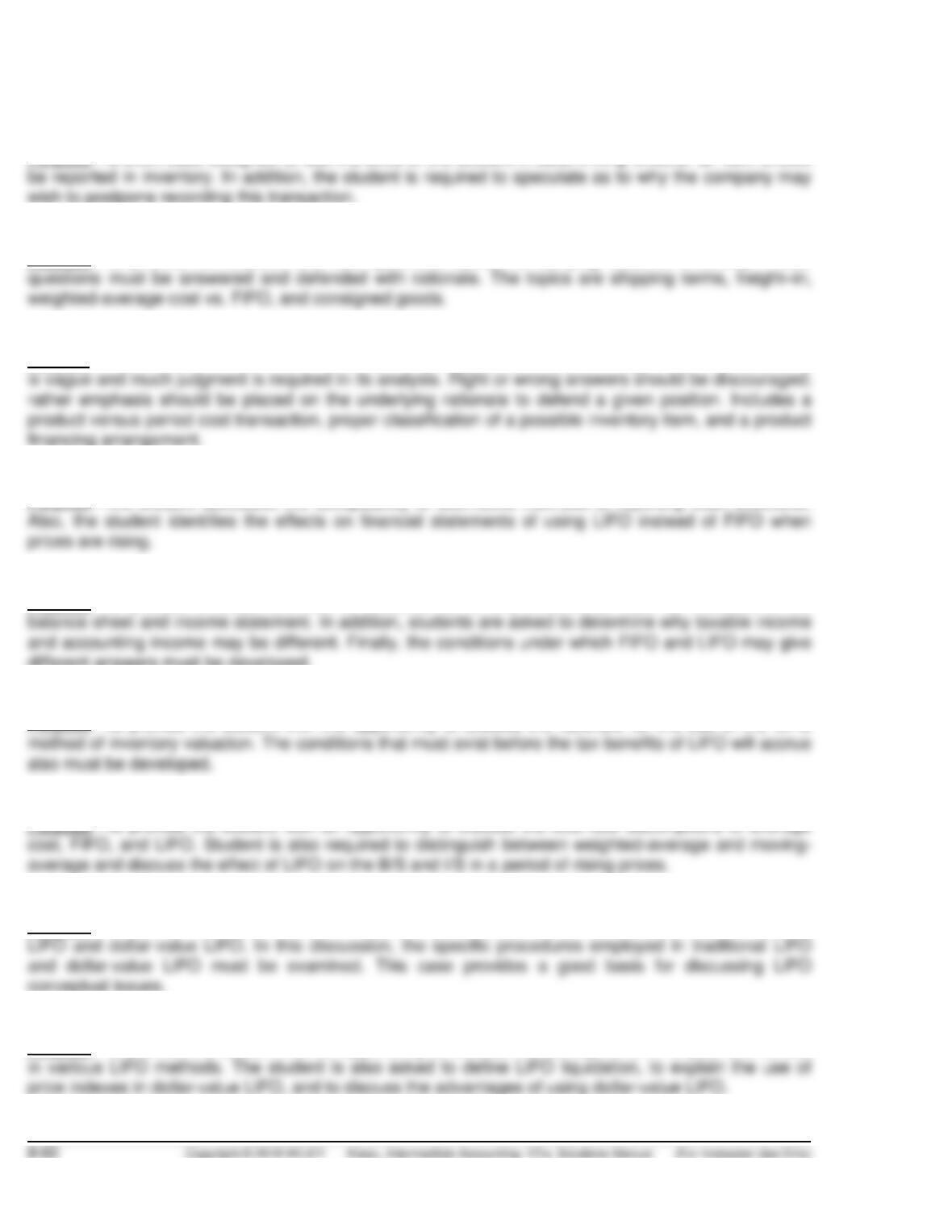
1. Refer to Schedule A. To express each year’s ending inventory (Column A)
in terms of base-year costs, simply divide the ending inventory by the
2. Next, compute the difference between the previous and the current
3. Finally, express this increment in current-year terms. For the second
year, this computation is straightforward: the base-year ending inven-
tory value is added to the difference in #2 above multiplied by the price
When valuing ending inventory, remember to include each yearly layer
adjusted by that year’s price index. Refer to Schedule B for 2019. Notice that
the +$9,000 change from the 2019 ending inventory indicates that the 2017
layer was not further eroded. Thus, ending inventory for 2019 would value
the first $80,000 worth of inventory at the base-year price index (1.00), the
next $10,000 (the remainder of the 2017 layer) at the 2017 price index (1.05),
and the last $9,000 at the 2019 price index (1.30).
TIME AND PURPOSE OF CONCEPTS FOR ANALYSIS
CA 8.1 (Time 15–20 minutes)
Purpose—a short case designed to test the skills of the student in determining whether an item should
wish to postpone recording this transaction.
CA 8.2 (Time 15–25 minutes)
Purpose—to provide the student with four questions about the carrying value of inventory. These
CA 8.3 (Time 25–35 minutes)
Purpose—to provide a number of difficult financial reporting transactions involving inventories. This case
CA 8.4 (Time 15–25 minutes)
Purpose—the student discusses the acceptability of alternative methods of reporting cash discounts.
CA 8.5 (Time 20–25 minutes)
Purpose—to provide a broad overview to students as to why inventories must be included in the
different answers must be developed.
CA 8.6 (Time 15–20 minutes)
Purpose—to provide the student with the opportunity to discuss the rationale for the use of the LIFO
CA 8.7 (Time 15–20 minutes)
CA 8.8 (Time 25–30 minutes)
Purpose—to provide the student with the opportunity to discuss the differences between traditional
CA 8.9 (Time 25–30 minutes)
Purpose—to provide the student with an opportunity to discuss the concept of a LIFO pool and its use