Accounting Chapter 8 Homework ESD Many Outlier Procedure Given Equation 829

166 CHAPTER 8/HYPOTHESIS TESTING: TWO SAMPLE INFERENCE

8.72 For hormone group 2, we note that the median dosage level is equal to the maximum dosage level and so

no patients could be classified as high-dose according the directions given. Instead we will denote low-

Two-Sample T-Test and CI: DBilPh_2, Below2

Two-Sample T-Test and CI: DPansec_2, Below2

Two-Sample T-Test and CI: DPanPh_2, Below2

Two-Sample T-Test and CI: DPansec_3, Below3

Two-Sample T-Test and CI: DBilPh_4, Below4

CHAPTER 8/HYPOTHESIS TESTING: TWO SAMPLE INFERENCE 167

Both use Pooled StDev = 2.8947

8.73 For each of the three age groups, we need to perform an F-test for equality of variances before performing a

Test for Equal Variances: FEV_1 versus Sex_1

Test for Equal Variances: FEV_2 versus Sex_2

Sex_2 N Lower StDev Upper

Two-Sample T-Test and CI: FEV_2, Sex_2

Sex_2 N Mean StDev SE Mean

Test for Equal Variances: FEV_3 versus Sex_3

Sex_3 N Lower StDev Upper

0 22 0.306335 0.412692 0.623310

Two-Sample T-Test and CI: FEV_3, Sex_3

Sex_3 N Mean StDev SE Mean

168 CHAPTER 8/HYPOTHESIS TESTING: TWO SAMPLE INFERENCE

8.74 For each of the 4 Age-Sex groups under investigation, we find no significant differences in variance of

FEV by smoking status, so we will perform t-tests assuming equal variance.

Test for Equal Variances: FEV_2-0 versus Smoke_2-0

Smoke_2-0 N Lower StDev Upper

Test for Equal Variances: FEV_2-1 versus Smoke_2-1

Smoke_2-1 N Lower StDev Upper

0 141 0.703331 0.79785 0.92039

Test for Equal Variances: FEV_3-0 versus Smoke_3-0

Smoke_3-0 N Lower StDev Upper

0 10 0.213362 0.326181 0.656815

Test for Equal Variances: FEV_3-1 versus Smoke_3-1

Smoke_3-1 N Lower StDev Upper

Two-Sample T-Test and CI: FEV_2-0, Smoke_2-0

Smoke_2-0 N Mean StDev SE Mean

0 114 2.837 0.429 0.040

Two-Sample T-Test and CI: FEV_2-1, Smoke_2-1

Smoke_2-1 N Mean StDev SE Mean

Two-Sample T-Test and CI: FEV_3-0, Smoke_3-0

CHAPTER 8/HYPOTHESIS TESTING: TWO SAMPLE INFERENCE 169

Two-Sample T-Test and CI: FEV_3-1, Smoke_3-1

Smoke_3-1 N Mean StDev SE Mean

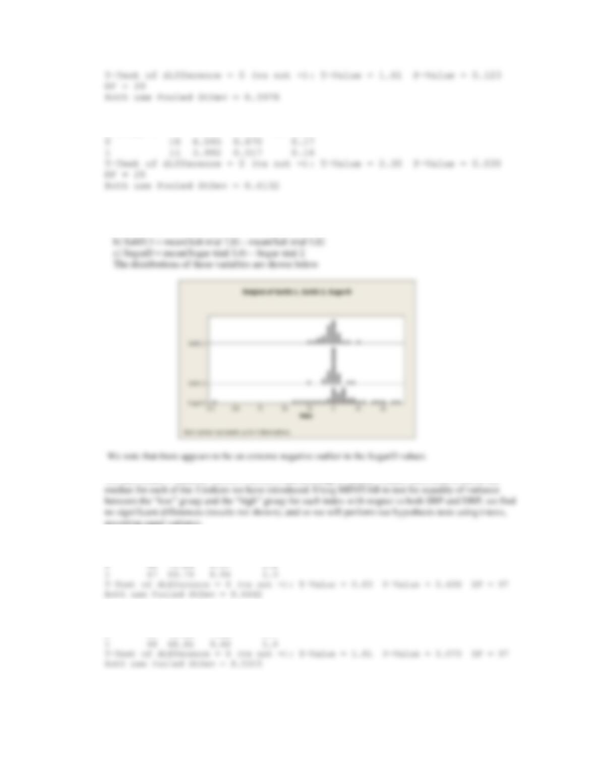
8.75 We will use the following 3 variables for the next two questions:

a) SaltD.1 = mean(Salt trial 3, 4) – mean(Salt trial 1,2)

We then create 3 variables: LowS.1, LowS.3, and LowSug, to denote whether each child is below the

assuming equal variance.

Two-Sample T-Test and CI: Mn_sbp, LowS.1

LowS.1 N Mean StDev SE Mean

Two-Sample T-Test and CI: Mn_sbp, LowS.3

LowS.3 N Mean StDev SE Mean

0 51 72.06 7.60 1.1

Two-Sample T-Test and CI: Mn_sbp, LowSug

LowSug N Mean StDev SE Mean

170 CHAPTER 8/HYPOTHESIS TESTING: TWO SAMPLE INFERENCE

Two-Sample T-Test and CI: Mn_dbp, LowS.3

LowS.3 N Mean StDev SE Mean

0 51 43.28 6.44 0.90

Two-Sample T-Test and CI: Mn_dbp, LowSug

LowSug N Mean StDev SE Mean

8.76 For this exercise, we compare the patients in the upper and lower quintiles of each measure. Will we

continue to assume equal variance for each of the t-tests. The variables QuinS.1, QuinS.3, and QuinSug

take the value 0 for babies scoring in the lowest quintile and take the value 1 for babies scoring the

highest quintile for a given index. Still we find no significant differences in SBP or DBP, suggesting that

these taste response indices are not related to blood pressure levels.

Two-Sample T-Test and CI: Mn_sbp, QuinS.1

QuinS.1 N Mean StDev SE Mean

0 18 69.4 10.1 2.4

Two-Sample T-Test and CI: Mn_sbp, QuinSug

QuinSug N Mean StDev SE Mean

0 20 68.30 8.82 2.0

CHAPTER 8/HYPOTHESIS TESTING: TWO SAMPLE INFERENCE 171

Two-Sample T-Test and CI: Mn_dbp, QuinS.3

QuinS.3 N Mean StDev SE Mean

0 20 42.92 8.84 2.0

Two-Sample T-Test and CI: Mn_dbp, QuinSug

QuinSug N Mean StDev SE Mean

0 20 41.33 5.40 1.2

8.77 The 95% CI

xrt

n1,.975

s

n

; this implies that the width of the 95% CI

2t

n1,.975

s

n

. Thus,

8.79 We should use a two sample t test with either equal or unequal variances. To assess which specific test to

8.80 We wish to test the hypothesis versus . We compute the

pooled variance estimate as follows

The pooled variance test statistic is given by

H01 2 1

2

:,

P

V

H11 2 1

2

:,

P

V

z

172 CHAPTER 8/HYPOTHESIS TESTING: TWO SAMPLE INFERENCE

8.81-8.84 Two key issues arise that are specific to this data set. First, we notice that missing values are coded as 9,

and so we must take care to handle them appropriately. Here, we will exclude missing values from our

One-Sample T: Dmax, D12, Dav, Dov

Test of mu = 0 vs not = 0

8.85 We will use the ESD Many Outlier Procedure given in Equation 8.29 (in Chapter 8, text). From Table

8.7, we see that for Full Scale IQ (IQF) in the control group, , s 15.3, n 78. We will attempt

to detect as many as 5 outliers (i.e., k 5). From Figure 8.12(a), since

x

Test Statistics and Critical Values for IQF, Control Group

ns p-value

78 92.9 15.3 141 3.136 NS

x

92 9.

x

n

 ESD n

 ESD ,.95n

ESD78 95,.

*

CHAPTER 8/HYPOTHESIS TESTING: TWO SAMPLE INFERENCE 173

8.86 We use the same approach as in Problem 8.85. We have the following test statistics and p-values:

Test Statistics and Critical Values for IQF, Exposed Group

ns p-value

46 88.0 12.2 46 3.443

8.87 We will perform a two-sample t test to compare mean IQF between exposed and control children. We

8.88 We will use the same procedure as in 8.85, for each of the 6 subgroups in question

Test Statistics and Critical Values for 5-9 year old boys

ns p-value

x

n

 ESD n

 ESD ,.95n

*.05

x

n

 ESD n

 ESD ,.95n

174 CHAPTER 8/HYPOTHESIS TESTING: TWO SAMPLE INFERENCE

Test Statistics and Critical Values for 10-14 year old boys

ns p-value

155 3.29 0.824 5.22 2.35 >3.52 NS

Test Statistics and Critical Values for 10-14 year old girls

ns p-value

Test Statistics and Critical Values for 15-19 year old boys

ns p-value

x

Using the ESD procedure, we find no outliers among the FEV values for any of the 6 subgroups.

8.89 The se of ln (ERG amplitude) . It reflects the error in the estimate of the mean

8.91 We have the test statistic

x

n

 ESD n

 ESD ,.95n

x

n

 ESD n

 ESD ,.95n

x

n

 ESD n

 ESD ,.95n

018 62 0023..

CHAPTER 8/HYPOTHESIS TESTING: TWO SAMPLE INFERENCE 175

The test statistic is given by

8.95 We wish to test the hypothesis vs. , where true mean change (follow up

minus baseline) in diastolic blood pressure. The test statistic is

8.96 To compare the mean DBP change in the two groups, we test the hypothesis

P

8.97 For this purpose, we complete the pooled variance estimate

H

d

00:

P

H

d

10:

P

z

P

d

t

176 CHAPTER 8/HYPOTHESIS TESTING: TWO SAMPLE INFERENCE

Therefore, we have the test statistic

8.98 We use the power formula

8.100 We have the test statistic

8.101 A 95% CI for d

P

is given by

8.102 We use the sample size formula (see chapter 7)

CHAPTER 8/HYPOTHESIS TESTING: TWO SAMPLE INFERENCE 177

8.103 We use the sample size formula based on a single sample of differences given by

Thus, we need to study 32 subjects to have 90% power.

8.104 We use the power formula

8.105 We use the power formula for comparing two mean differences given by

Power ) z1

D

/2 ‘

V

1

2n1

V

2

2n2

§

©

¨

·

¹

¸

178 CHAPTER 8/HYPOTHESIS TESTING: TWO SAMPLE INFERENCE

8.109 We use the sample size formula

8.110 A 95% CI for

P

is given by .

8.111 There is in fact overlap between the 95% CI’s for

P

for I and U plants. However, this does not mean that

P

I

8.112 We wish to test the hypothesis vs. . We will use a two sample t test to test this

8.113 We first compute the pooled variance estimate

xt sr7975 8

,.

H

U

I

0:

P

H

U

I

1:

P

z

CHAPTER 8/HYPOTHESIS TESTING: TWO SAMPLE INFERENCE 179

We then have the test statistic

8.115 In order to test the null hypothesis that mean baseline creatinine levels would be the same in the NAPAP

Test for Equal Variances: creat_68 versus control

Two-Sample T-Test and CI: creat_68_1, creat_68_3

8.116 Since we are now comparing each of the two NAPAP groups with the control group, we should against