8-57
2. Describe how Gallo’s control of variable manufacturing overhead items differs from its
control of fixed manufacturing overhead items.
SOLUTION
8-58
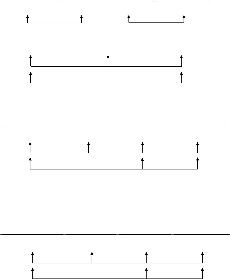
SOLUTION EXHIBIT 8-38
Actual Costs
Incurred
(Actual Input Qty.
Actual Rate)
Actual Input Qty.
Budgeted Rate
Purchases Usage
Flexible Budget:
Budgeted Input Qty.
Allowed for
Actual Output
Budgeted Rate
Direct
Materials
163,000 $10.40
$1,695,200
163,000 $11.50
$1,874,500
126,600 $11.50
$1,455,900
6 20,000 $11.50
$1,380,000
Direct
Manuf.
Labor
21,000 $25.50
$535,500
21,000 $25
$525,000
19,190 $25
$479,750
Actual Costs
Incurred
Actual Input Qty.
Actual Rate
Actual Input Qty.
Budgeted Rate
Flexible Budget:
Budgeted Input Qty.
Allowed for
Actual Output
Budgeted Rate
Allocated:
Budgeted Input Qty.
Allowed for
Actual Output
Budgeted Rate
Variable
MOH
21,000 $9.63
$202,300
21,000 $10
$210,000
19,190 $10
$191,900
19,190 $10
$191,900
Actual Costs
Incurred
(1)
Same Budgeted
Lump Sum
(as in Static Budget)
Regardless of
Output Level
(2)
Flexible Budget:
Same Budgeted
Lump Sum
(as in Static Budget)
Regardless of
Output Level
(3)
Allocated:
Budgeted Input Qty.
Allowed for
Actual Output
× Budgeted Rate
(4)
Fixed
MOH
$957,550
$1,000,000
50,000 × $20
$1,000,000
19,190× $20
$383,800
$179,300 F
Price variance
$75,900 U
Efficiency variance
$10,500 U
Price variance
$55,750 U
Efficiency variance
$66,250 U
Flexible-budget variance
$7,700 F
Spending variance
$18,100 U
Efficiency
Never a variance
$10,400 U
Flexible-budget variance
Never a variance
$616,200 U
$42,450 F
Flexible-budget variance
$616,200 U
Production volume variance
Never a variance
$42,450 F
Spending variance
8-59
8-39 (30−50 min.) Review of Chapters 7 and 8, 3-variance analysis.
(CPA, adapted) The Brown Manufacturing Company’s costing system has two direct-cost
categories: direct materials and direct manufacturing labor. Manufacturing overhead (both
variable and fixed) is allocated to products on the basis of standard direct manufacturing labor–
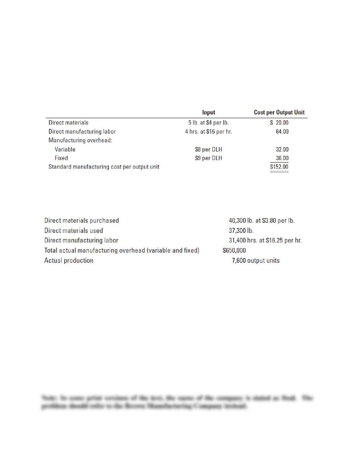
hours (DLH). At the beginning of 2014, Beal adopted the following standards for its
manufacturing costs:
The denominator level for total manufacturing overhead per month in 2014 is 37,000 direct
manufacturing labor-hours. Beal’s flexible budget for January 2014 was based on this
denominator level. The records for January indicated the following:
Required:
1. Prepare a schedule of total standard manufacturing costs for the 7,600 output units in January
2014.
2. For the month of January 2014, compute the following variances, indicating whether each is
favorable (F) or unfavorable (U):
a. Direct materials price variance, based on purchases
b. Direct materials efficiency variance
c. Direct manufacturing labor price variance
d. Direct manufacturing labor efficiency variance
e. Total manufacturing overhead spending variance
f. Variable manufacturing overhead efficiency variance
g. Production-volume variance
SOLUTION
8-60
8-61
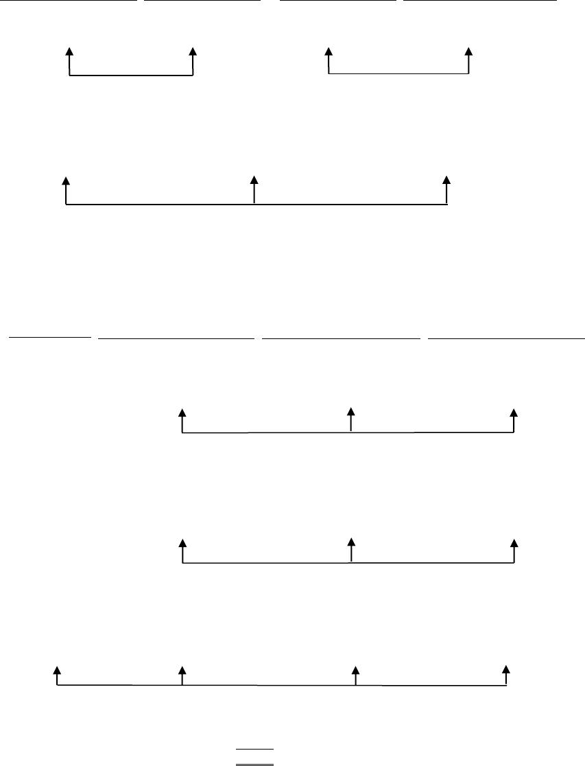
SOLUTION EXHIBIT 8-39
Actual Costs
Incurred:
Actual Input Qty.
Actual Input Qty.
Budgeted Price
Flexible Budget:
Budgeted Input Qty.
Allowed for
Actual Output
× Actual Rate
Purchases
Usage
× Budgeted Price
Direct
Materials
(40,300 $3.80)
$153,140
(40,300 $4.00)
$161,200
(37,300 $4.00)
$149,200
(38,000 $4.00)
$152,000
$8,060 F $2,800 F
a. Price variance b. Efficiency variance
Direct
Manuf.
Labor
(31,400 $16.25)
$510,250
(31,400 $16.00)
$502,400
(30,400 $16.00)
$486,400
$7,850 U $16,000 U
c. Price variance d. Efficiency variance
Actual
Costs
Incurred
Actual Input Qty.
Budgeted Rate
Flexible Budget:
Budgeted Input Qty.
Allowed for
Actual Output
Budgeted Rate
Allocated:
(Budgeted Input Qty.
Allowed for
Actual Output
Budgeted Rate)
Variable
Manuf.
Overhead
(not given)
(31,400 $8.00)
$251,200
(30,400 $8.00)
$243,200
(30,400 $8.00)
$243,200
$8,000 U
Efficiency variance Never a variance
Fixed
Manuf.
Overhead
(not given)
$333,000
$333,000
(30,400 $9.00)
$273,600
$59,400 U*
Never a variance Prodn. volume variance
Total
Manuf.
Overhead
(given)
$650,000
($333,000 + $251,200)
$584,200
($243,200 + $333,000)
$576,200
($234,200 + $273,600)
$507,800
$65,800 U $8,000 U $59,400 U
e. Spending variance f. Efficiency variance g. Prodn. volume variance
*Denominator level in hours 37,000
Production volume in standard hours allowed 30,400
Production-volume variance 6,600 hours × $9.00 = $59,400 U
8-62
8-40 (20 minutes) Non-financial variances.
Max Canine Products produces high-quality dog food distributed only through veterinary offices.
To ensure that the food is of the highest quality and has taste appeal, Max Canine has a rigorous
inspection process. For quality control purposes, Max Canine has a standard based on the pounds
of food inspected per hour and the number of pounds that pass or fail the inspection.
Max Canine expects that for every 13,000 pounds of food produced, 1,300 pounds of food
will be inspected. Inspection of 1,300 pounds of dog food should take 1 hour. Max Canine also
expects that 5% of the food inspected will fail the inspection. During the month of May,
Supreme produced 2,990,000 pounds of food and inspected 292,500 pounds of food in 200
hours. Of the 292,500 pounds of food inspected, 15,625 pounds of food failed to pass the
inspection.
Required:
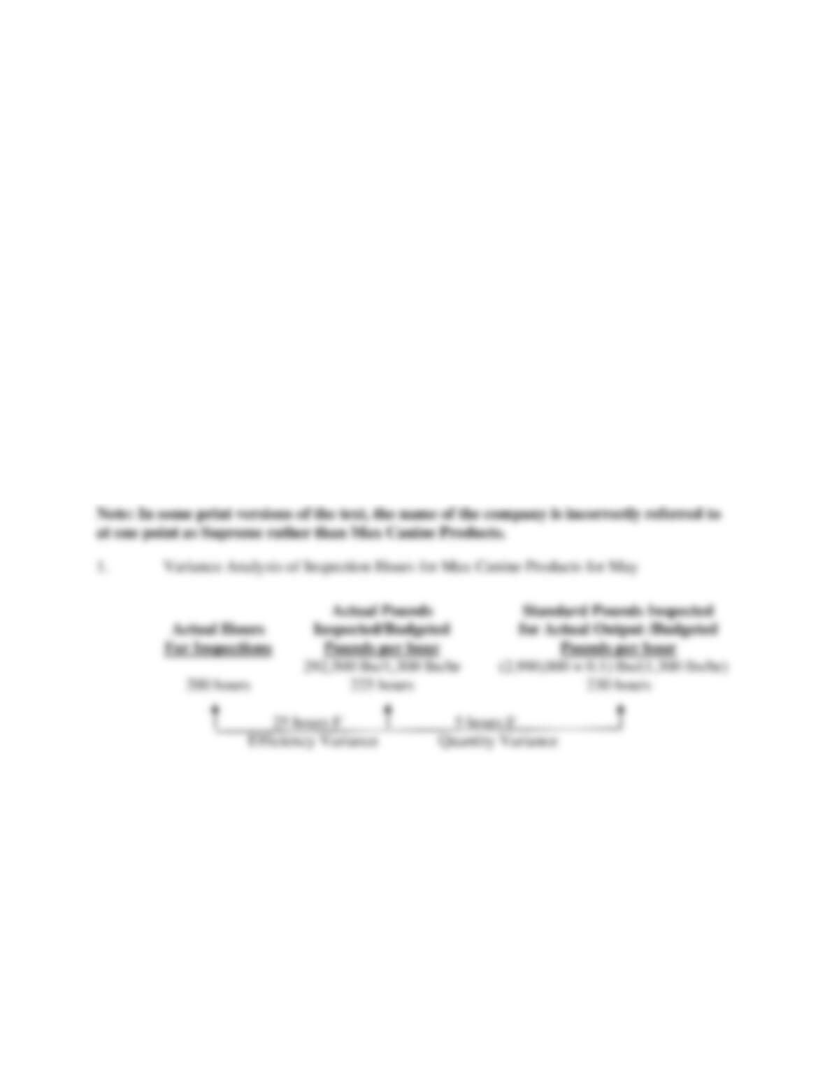
1. Compute two variances that help determine whether the time spent on inspections was more
or less than expected. (Follow a format similar to the one used for the variable overhead
spending and efficiency variances, but without prices.)
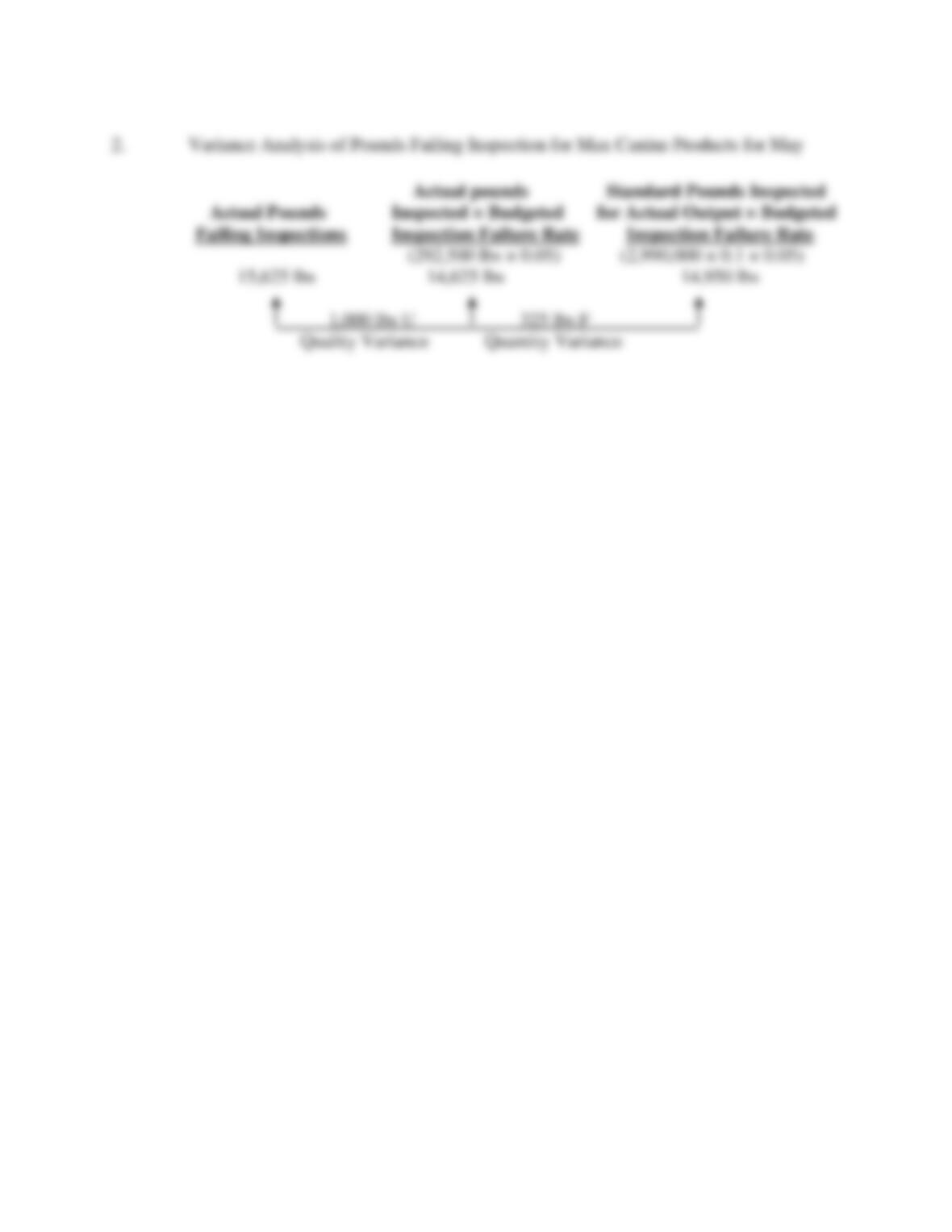
2. Compute two variances that can be used to evaluate the percentage of the food that fails the
inspection.
SOLUTION
8-63
8-41 (30 minutes) Overhead variances, service sector.
Cavio is a cloud service provider that offers computing resources to handle enterprise-wide
applications. For March 2014, Cavio estimates that it will provide 18,000 RAM hours of services
to clients. The budgeted variable overhead rate is $6 per RAM hour.
At the end of March, there is a $500 favorable spending variance for variable overhead and a
$1,575 unfavorable spending variance for fixed overhead. For the services actually provided
during the month, 14,850 RAM hours are budgeted and 15,000 RAM hours are actually used.
Total actual overhead costs are $119,875.
Required:
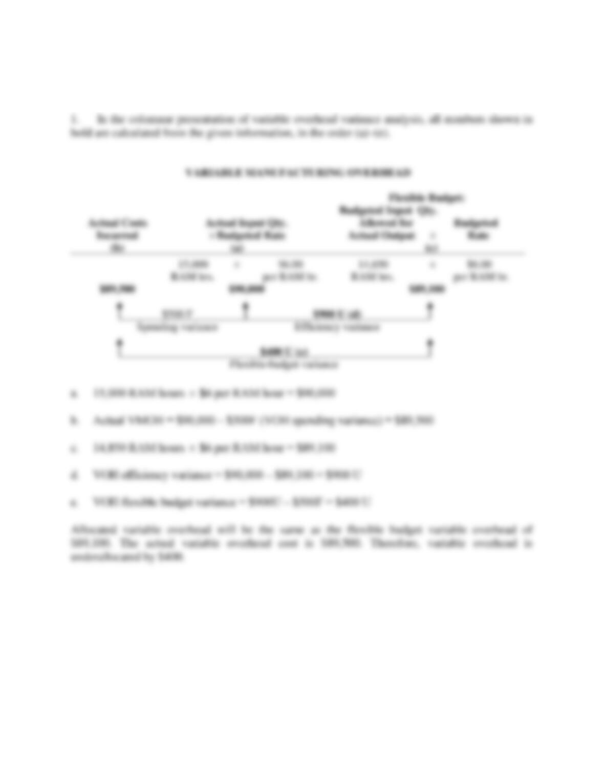
1. Compute efficiency and flexible-budget variances for Cavio’s variable overhead in March
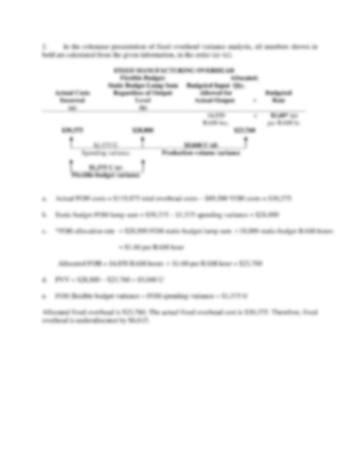
2014. Will variable overhead be over- or underallocated? By how much?
2. Compute production-volume and flexible–budget variances for Cavio’s fixed overhead in
March 2014. Will fixed overhead be over- or underallocated? By how much?
8-64
SOLUTION
8-65
8-66
8-42 (30 min.) Direct-cost and overhead variances, income statement.
The Kordell Company started business on January 1, 2013, in Raleigh. The company adopted a
standard absorption costing system for its one product—a football for use in collegiate
intramural sports. Because of the extensive handcrafting needed to do quality assurance on the
final product, Kordell chose direct labor as the application base for overhead and decided to use
the proration method to account for variances at year-end.
Kordell expected to make and sell 80,000 footballs the first year; each football was budgeted
to use 1 pound of leather and require 15 minutes of direct labor work. The company expected to
pay $1 for each pound of leather and compensate workers at an hourly wage of $16. Kordell has
no variable overhead costs, but expected to spend $200,000 on fixed manufacturing overhead in
2013.
In 2013, Kordell actually made 100,000 footballs and sold 80,000 of them for a total revenue
of $1 million.
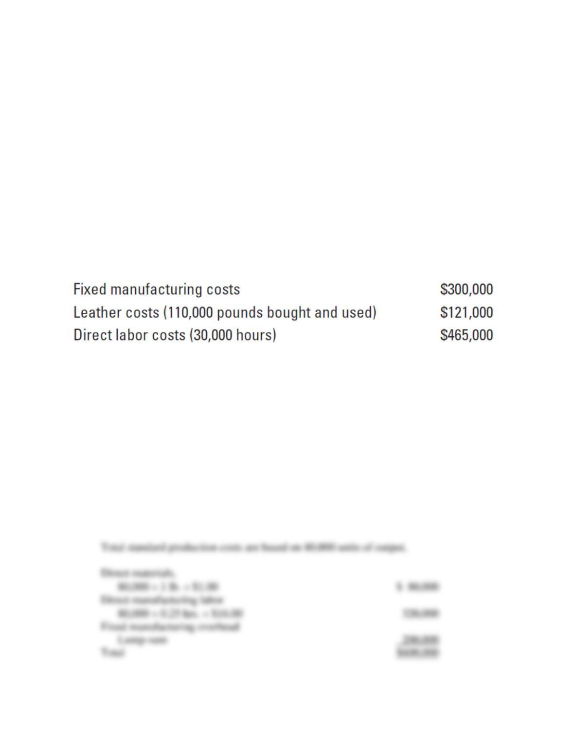
The expenses incurred were as follows:
Required:
1. Compute the following variances for 2013, and indicate whether each is favorable (F) or
unfavorable (U):
a. Direct materials efficiency variance
b. Direct materials price variance
c. Direct labor efficiency variance
d. Direct labor price variance
e. Total manufacturing overhead spending variance
f. Fixed overhead flexible budget variance
g. Fixed overhead production-volume variance
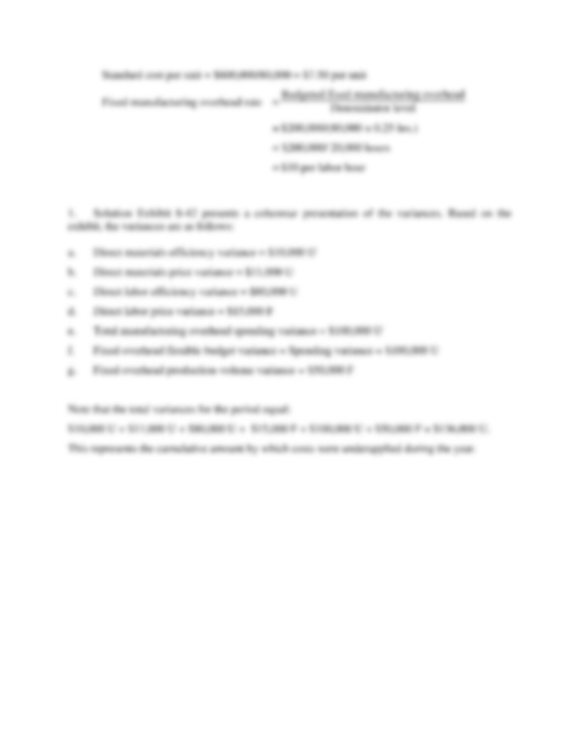
2. Compute Kordell Company’s gross margin for its first year of operation.
SOLUTION
8-67
8-68
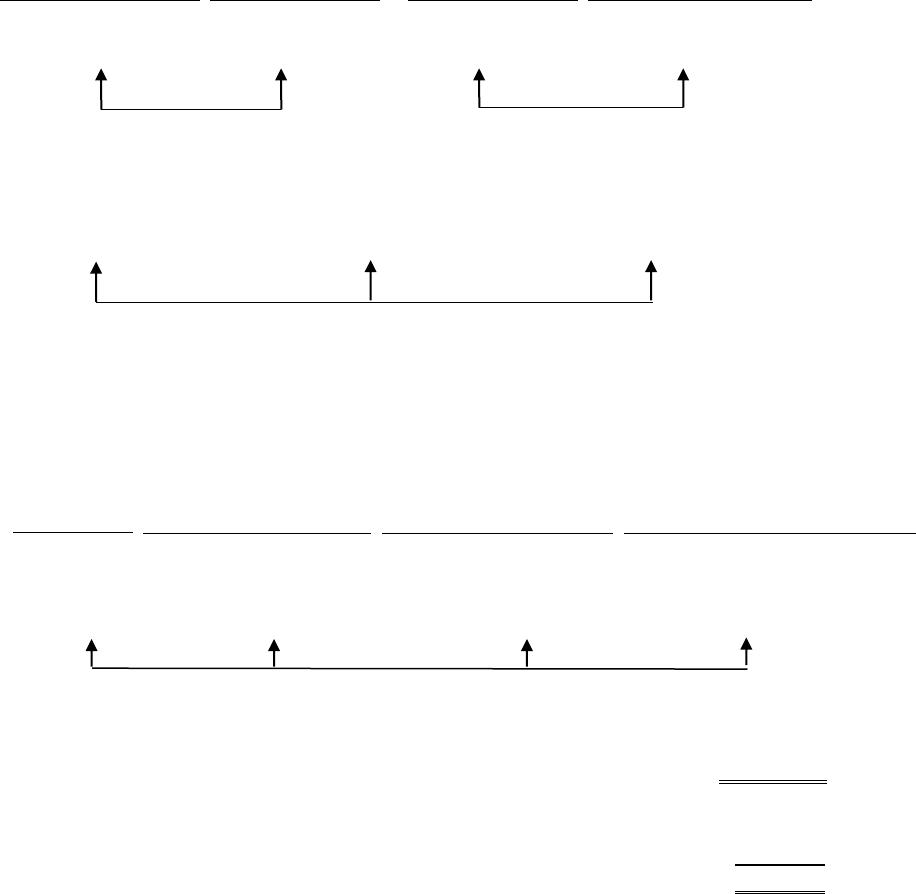
SOLUTION EXHIBIT 8-42
Actual Costs
Incurred:
Actual Input Qty.
Actual Input Qty.
Budgeted Price
Flexible Budget:
Budgeted Input Qty.
Allowed for
Actual Output
× Actual Rate
Purchases
Usage
× Budgeted Price
Direct
Materials
(110,000 $1.10)
$121,000
(110,000 $1)
$110,000
(110,000 $1)
$110,000
(100,000 1 lb. $1)
$100,000
$11,000 U $10,000 U
Price variance Efficiency variance
Direct
Manuf.
Labor
(30,000 $15.50)
$465,000
(30,000 $16.00)
$480,000
100,000 0.25 hrs $16.00)
$400,000
$15,000 F $80,000 U
Price variance Efficiency variance
Actual
Costs
Incurred
Actual Input Qty.
Budgeted Rate
Flexible Budget:
Budgeted Input Qty.
Allowed for
Actual Output
Budgeted Rate
Allocated:
(Budgeted Input Qty.
Allowed for
Actual Output
Budgeted Rate)
Fixed
Manuf.
Overhead
$300,000
$200,000
$200,000
(100,000 0.25 hrs $10.00)
$250,000
$100,000 U $50,000 F
Spending variance Never a variance Prodn. volume variance
2. Sales Revenue = 80,000 units sold × $12.50 = $1,000,000
Cost of Goods sold: At standard: 80,000 × $7.50 = $600,000
(+) Prorated share of underapplied cost: $136,000 × (80,000/100,000) = $108,800
Total $708,800
Gross Margin = $1,000,000 (–) $708,800
= $291,200

8-69
8-43 (40 – 50 minutes) Overhead variances, ethics
Hartmann Company uses standard costing. The company has two manufacturing plants, one in
Georgia and the other in Alabama. For the Georgia plant, Hartmann has budgeted annual output
of 2,000,000 units. Standard labor-hours per unit are 0.50, and the variable overhead rate for the
Georgia plant is $3.30 per direct labor-hour. Fixed overhead for the Georgia plant is budgeted at
$2,400,000 for the year.
For the Alabama plant, Hartmann has budgeted annual output of 2,100,000 units with
standard labor-hours also 0.50 per unit. However, the variable overhead rate for the Alabama
plant is $3.10 per hour, and the budgeted fixed overhead for the year is only $2,205,000.
Firm management has always used variance analysis as a performance measure for the two
plants and has compared the results of the two plants.
Tom Saban has just been hired as a new controller for Hartmann. Tom is good friends with
the Alabama plant manager and wants him to get a favorable review. Tom suggests allocating the
firm’s budgeted common fixed costs of $3,150,000 to the two plants, but on the basis of one-
third to the Alabama plant and two- thirds to the Georgia plant. His explanation for this
allocation base is that Georgia is a more expensive state than Alabama.
At the end of the year, the Georgia plant reported the following actual results: output of
1,950,000 using 1,020,000 labor-hours in total, at a cost of $3,264,000 in variable overhead and
$2,440,000 in fixed overhead.
Actual results for the Alabama plant are an output of 2,175,000 units using 1,225,000 labor-
hours with a variable cost of $3,920,000 and fixed overhead cost of $2,300,000. The actual
common fixed costs for the year were $3,075,000.
Required:
1. Compute the budgeted fixed cost per labor-hour for the fixed overhead separately for each
plant:
a. Excluding allocated common fixed costs
b. Including allocated common fixed costs
2. Compute the variable overhead spending variance and the variable overhead efficiency
variance separately for each plant.
3. Compute the fixed overhead spending and volume variances for each plant:
a. Excluding allocated common fixed costs
b. Including allocated common fixed costs
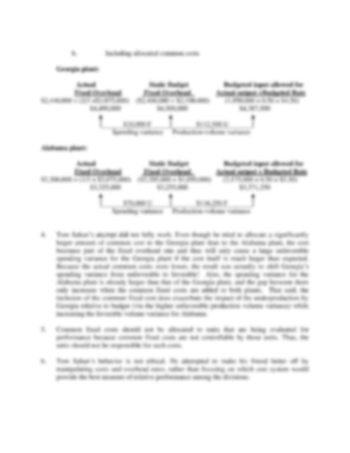
4. Did Tom Saban’s attempt to make the Alabama plant look better than the Georgia plant by
allocating common fixed costs work? Why or why not?
5. Should common fixed costs be allocated in general when variances are used as performance
measures? Why or why not?
6. What do you think of Tom Saban’s behavior overall?
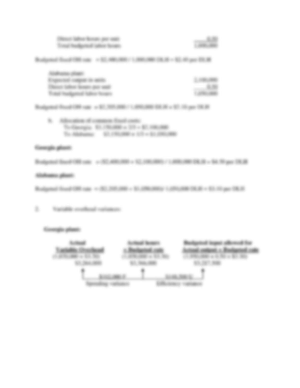
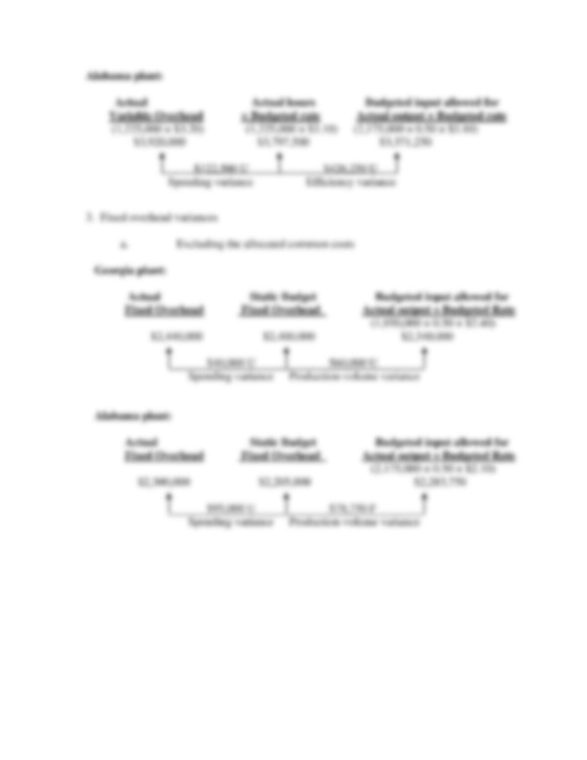
SOLUTION
8-70
8-71
8-72