Chapter 8
Flexible Budgets, Standard Costs, and
Variance Analysis
Solutions to Questions
8-1 The planning budget is prepared for the
planned level of activity. It is static because it is
8-2 A flexible budget can be adjusted to
reflect any level of activity—including the actual
level of activity. By contrast, a static planning
budget is prepared for a single level of activity
and is not subsequently adjusted.
8-3 Actual results can differ from the budget
for many reasons. Very broadly speaking, the
8-4 From a manager’s perspective,
differences between the planning budget and
actual results that are due to a change in
activity are very different from variances that are
8-5 A revenue variance is the difference
between how much the revenue should have
been, given the actual level of activity, and the
actual revenue for the period. A revenue
because the revenue is less than expected for
the actual level of activity.
given the actual level of activity, and the actual
amount of the cost. Like the revenue variance,
the interpretation of a spending variance is
straight-forward. A favorable spending variance
occurs because the cost is lower than expected
for the actual level of activity. An unfavorable
spending variance occurs because the cost is
higher than expected for the actual level of
happened at the actual level of activity to what
actually happened. A planning budget does not
enable these comparisons because it is based on
the planned level of activity rather than the
may be a function of the second cost driver, and
some costs may be a function of both cost
drivers.
8-10 Separating a spending variance into a
price variance and a quantity variance provides
8-11 The materials price variance is usually
the responsibility of the purchasing manager.
8-12 The materials price variance can be
computed either when materials are purchased
or when they are placed into production. It is
8-13 This combination of variances may
indicate that inferior quality materials were
purchased at a discounted price, but the low-
quality materials created production problems.
8-14 Several factors other than the
contractual rate paid to workers can cause a
labor rate variance. For example, skilled workers
8-15 If poor quality materials create
production problems, a result could be excessive
labor time and therefore an unfavorable labor
efficiency variance. Poor quality materials would
not ordinarily affect the labor rate variance.
8-16 If overhead is applied on the basis of
direct labor-hours, then the variable overhead
comparing the number of direct labor-hours
actually worked to the standard hours allowed.
Only the “SR” part of the formula, the standard
rate, differs between the two variances.
output of the entire system is limited by the
capacity of the bottleneck. If workstations
before the bottleneck in the production process
The Foundational 15
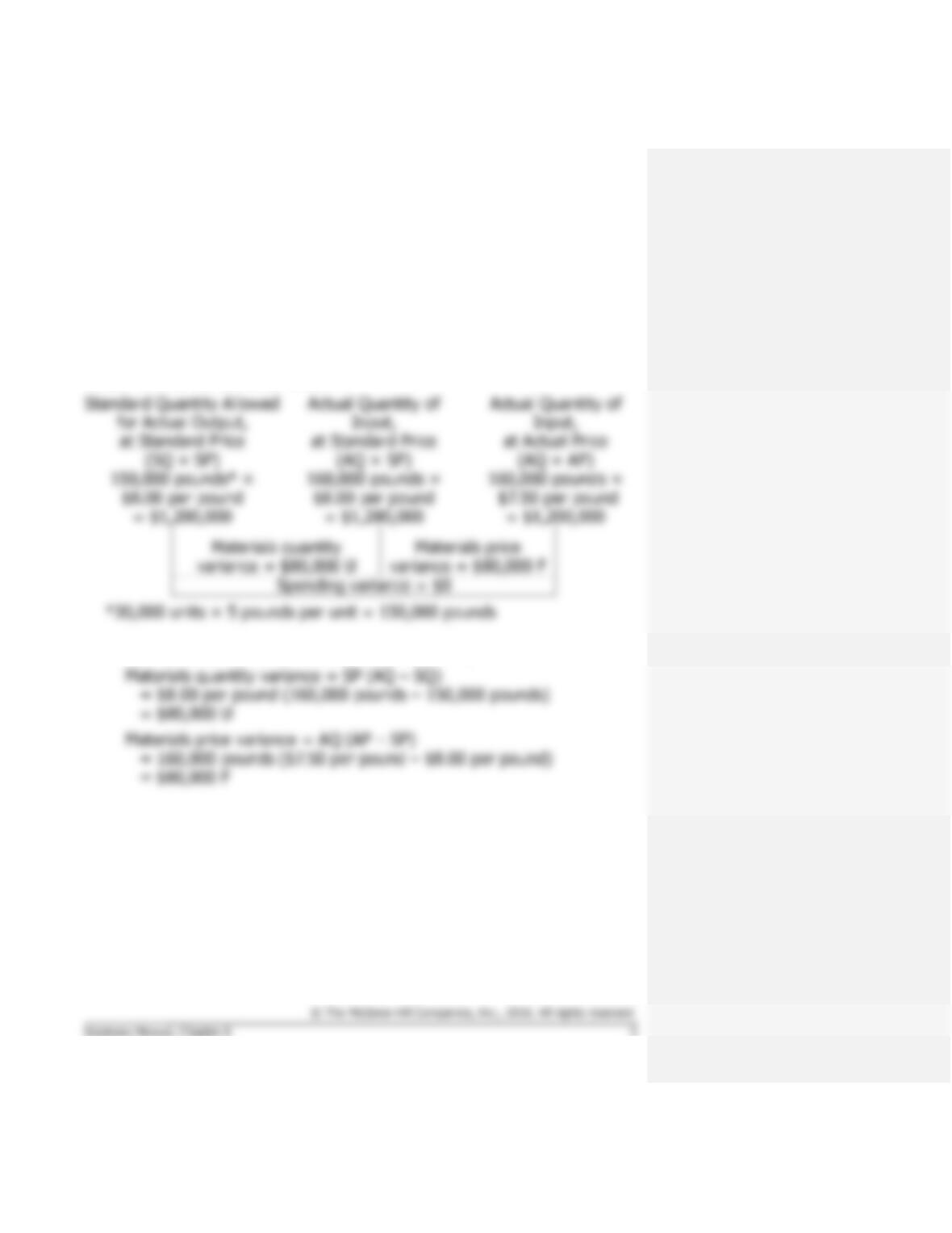
1., 2., and 3.
The raw materials cost included in the flexible budget (SQ × SP =
$1,200,000), the materials quantity variance ($80,000 U), and the
materials price variance ($80,000 F) can be computed using the general
model for cost variances as follows:
Alternatively, the variances can be computed using the formulas:
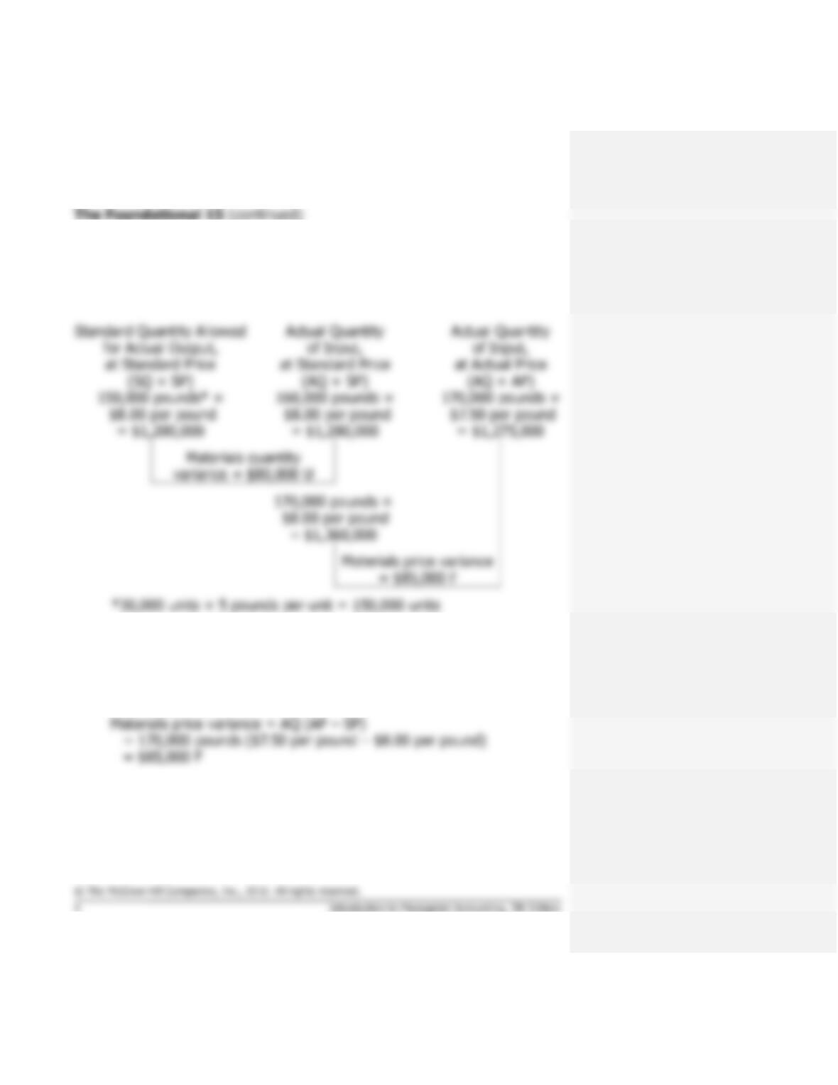
4. and 5.
The materials quantity variance ($80,000 U), and the materials price
variance ($85,000 F) can be computed as follows:
Alternatively, the variances can be computed using the formulas:
Materials quantity variance = SP (AQ – SQ)
= $8.00 per pound (160,000 pounds – 150,000 pounds)
= $80,000 U
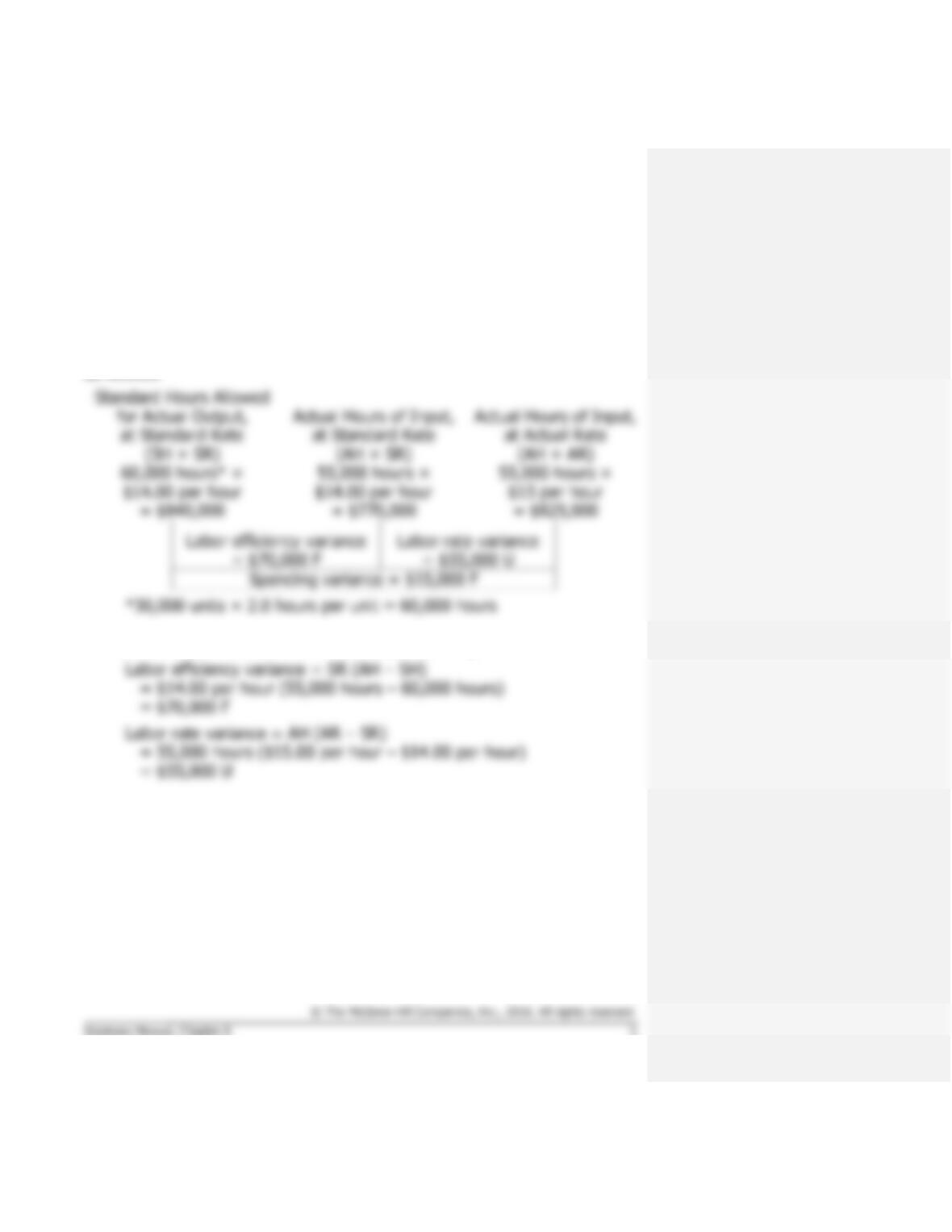
The Foundational 15 (continued)
6., 7., and 8.
The direct labor cost included in the flexible budget (SH × SR = $840,000),
the labor efficiency variance ($70,000 F), and the labor rate variance
($55,000 U) can be computed using the general model for cost variances
as follows:
Alternatively, the variances can be computed using the formulas:
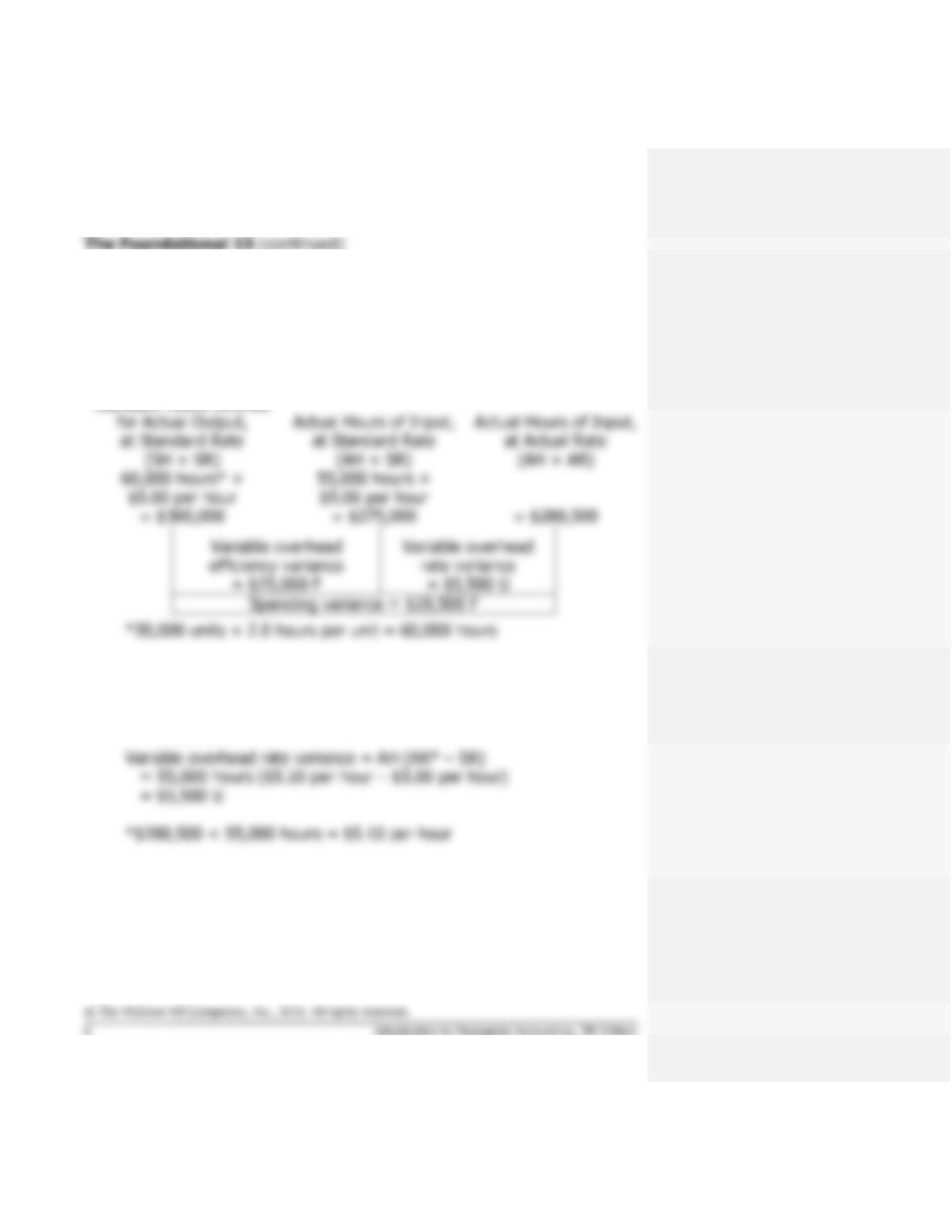
9., 10., and 11.
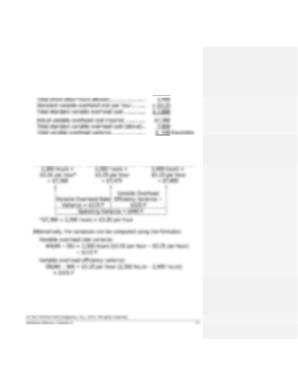
The variable overhead cost included in the flexible budget (SH × SR =
$300,000), the variable overhead efficiency variance ($25,000 F), and the
variable overhead rate variance ($5,500 U) can be computed using the
general model for cost variances as follows:
Standard Hours Allowed
Alternatively, the variances can be computed using the formulas:
Variable overhead efficiency variance = SR (AH – SH)
= $5.00 per hour (55,000 hours – 60,000 hours)
= $25,000 F
The Foundational 15 (continued)
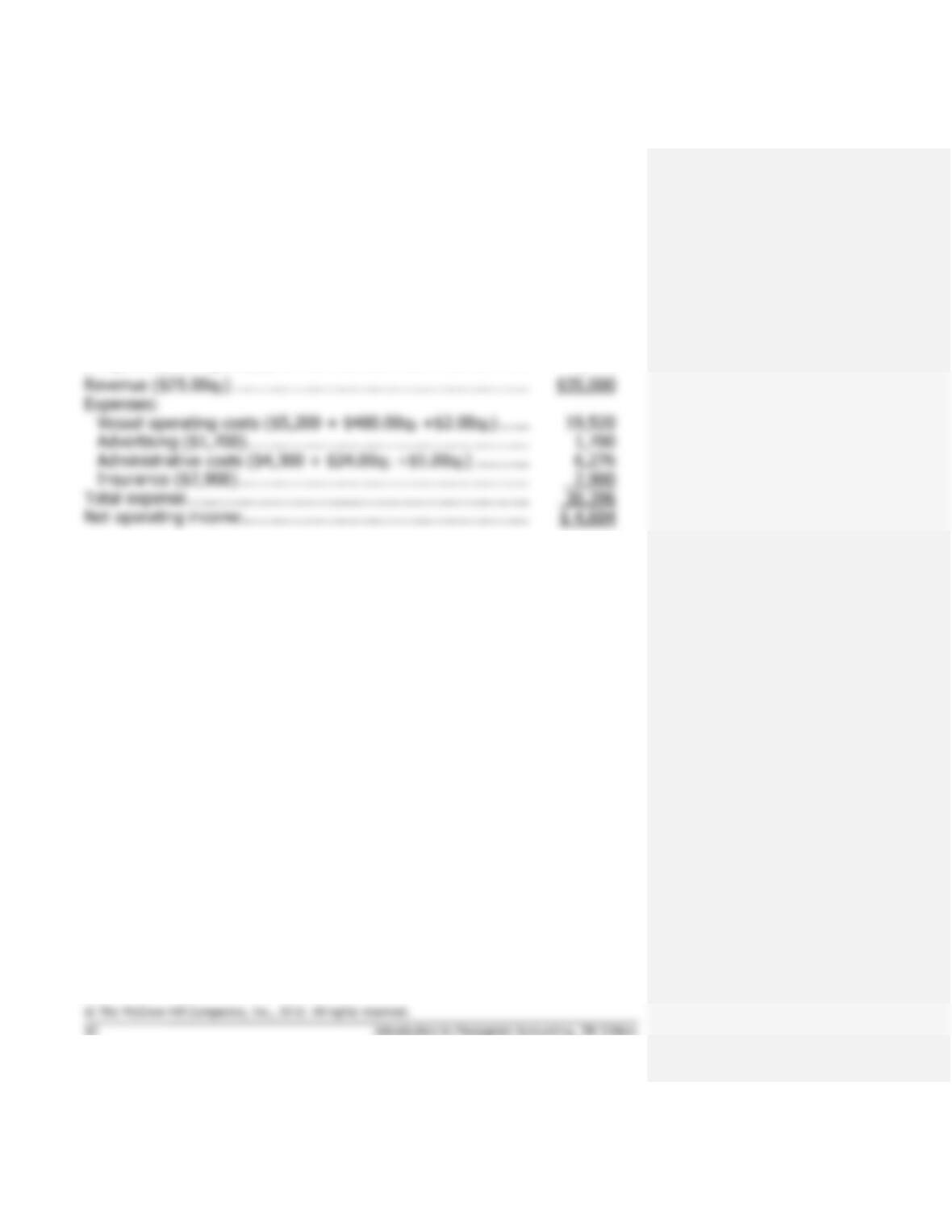
12. The amounts included in the flexible budget are computed as follows:
Preble Company
Flexible Budget
For the Month Ended March 31
Units sold (
q
) …………………………………………………….
30,000
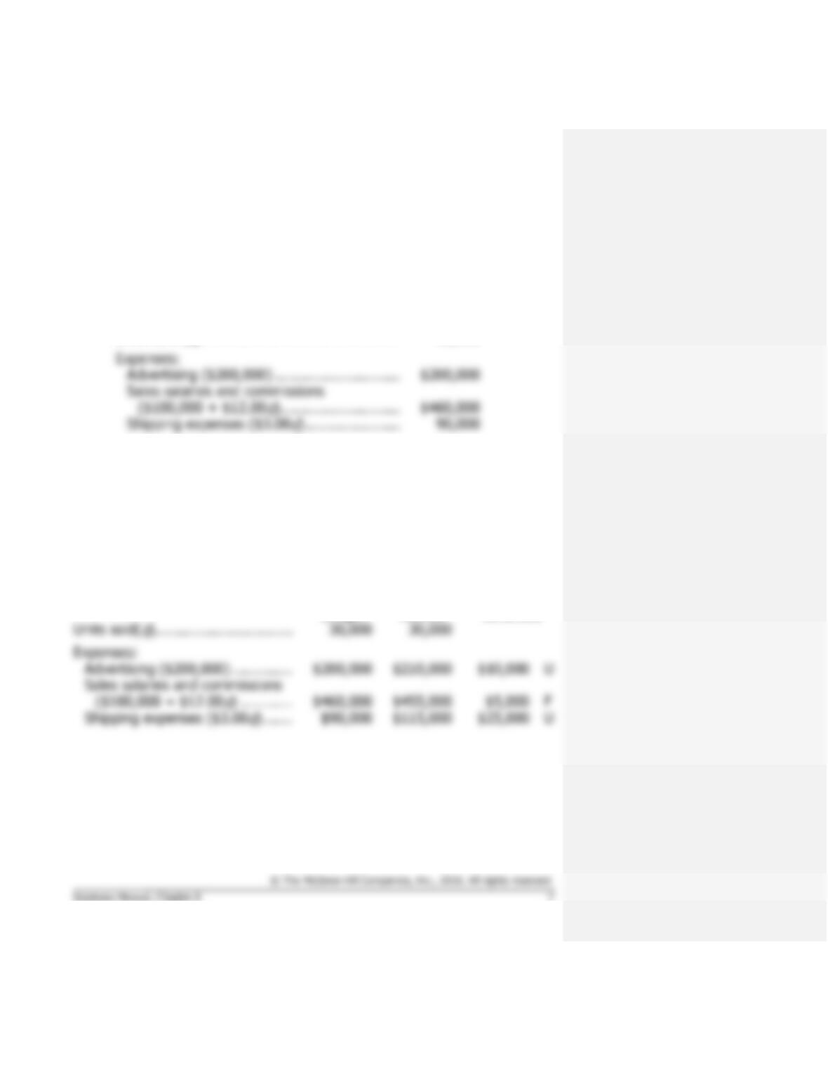
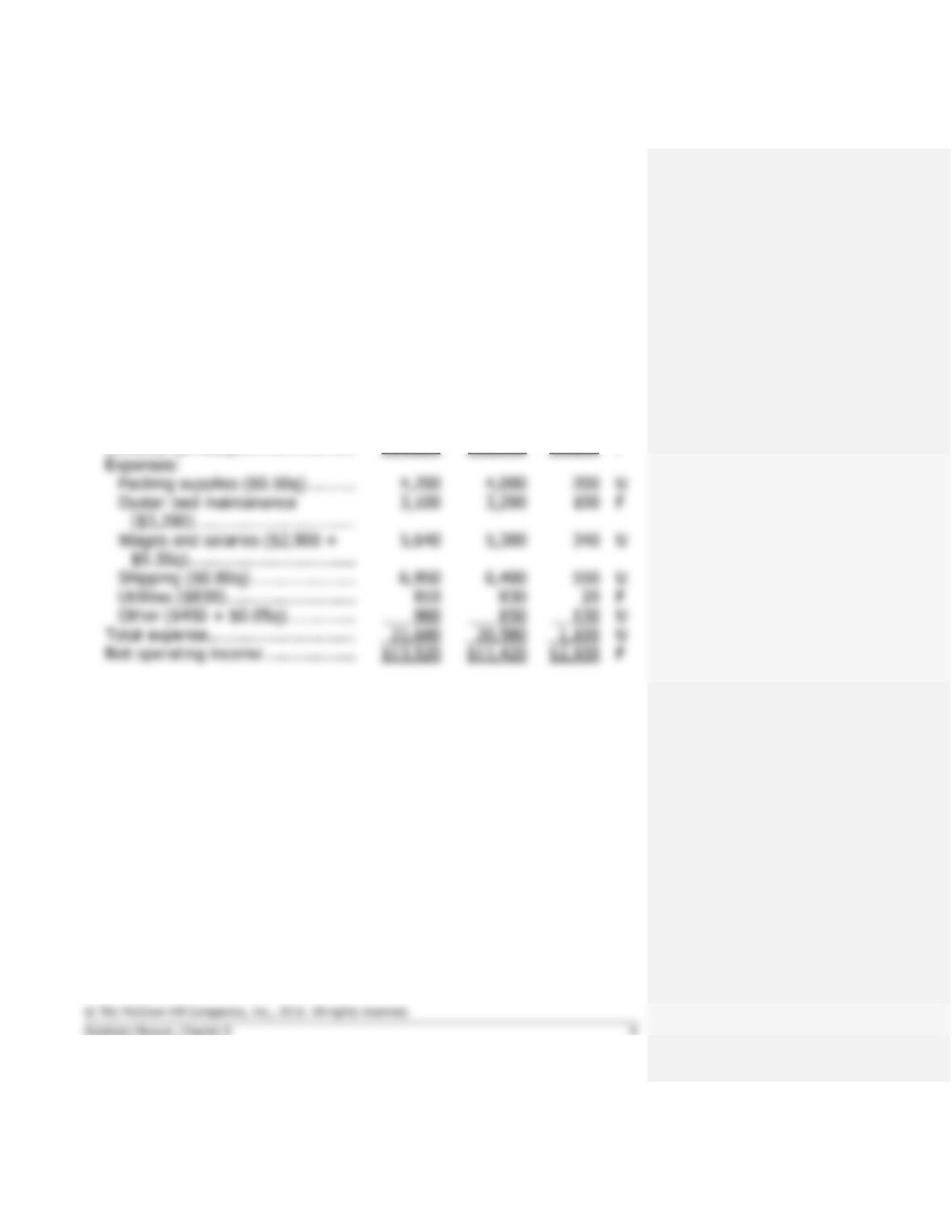
13., 14., and 15.
The spending variances for advertising ($), sales salaries and commissions
($), and shipping expenses ($) are computed as follows:
Preble Company
Spending Variances
For the Month Ended March 31
Flexible
Budget
Actual
Results
Spending
Variances
Expenses:
F
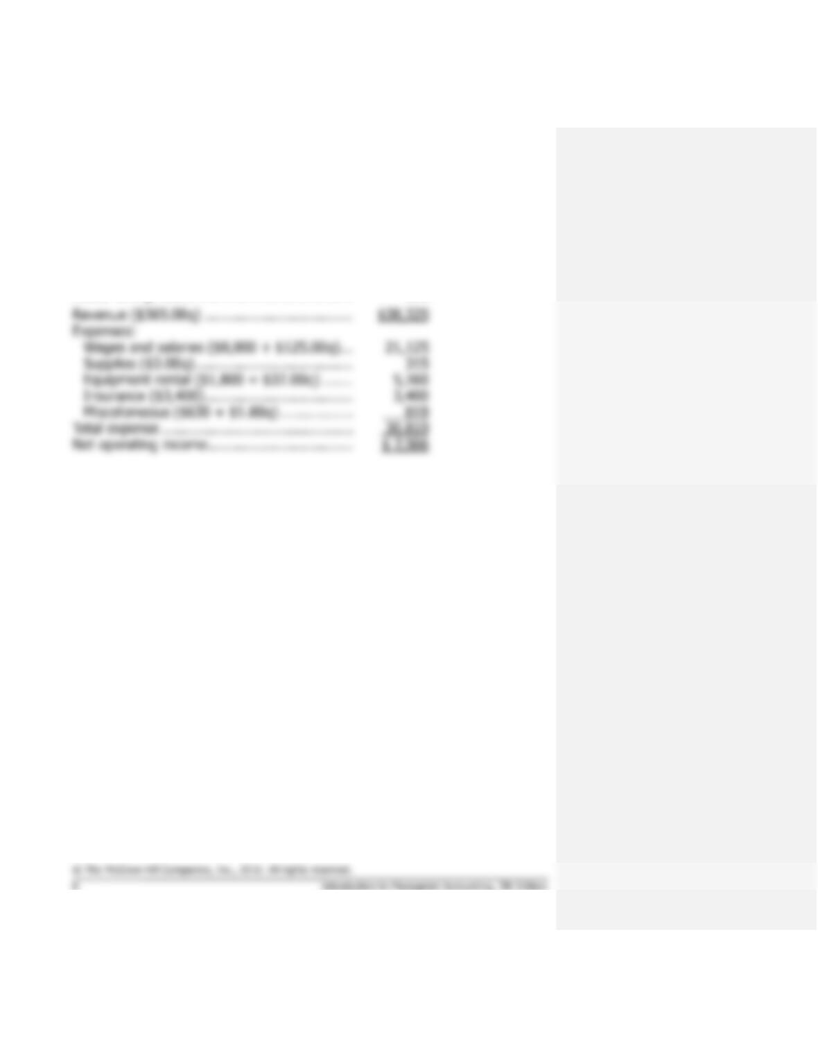
Exercise 8-1 (10 minutes)
Puget Sound Divers
Flexible Budget
For the Month Ended May 31
Actual diving-hours ……………………………….
105
Net operating income …………………………….
Exercise 8-2 (15 minutes)
Quilcene Oysteria
Revenue and Spending Variances
For the Month Ended August 31
Actual
Results
Flexible
Budget
Revenue
and
Spending
Variances
Pounds …………………………………
8,000
8,000
Revenue ($4.00q) ……………………
$35,200
$32,000
$3,200
F
Expenses:
F
850
130
U
Net operating income ………………
F
Exercise 8-3 (15 minutes)
Alyeski Tours
Planning Budget
For the Month Ended July 31
Budgeted cruises (q1) ………………………………………………….
24
Budgeted passengers (q2) …………………………..……………….
1,400
6,276
Net operating income ………………………………………………….
Exercise 8-4 (20 minutes)
1.
Number of helmets …………………………………….
35,000
Standard kilograms of plastic per helmet …………
× 0.6
Total standard kilograms allowed …………………..
Standard cost per kilogram …………………………..
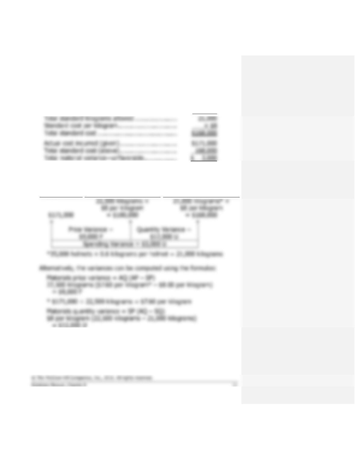
2.
Actual Quantity
of Input, at
Actual Price
Actual Quantity of Input,
at Standard Price
Standard Quantity
Allowed for Output, at
Standard Price
(AQ × AP)
(AQ × SP)
(SQ × SP)
Exercise 8-5 (20 minutes)
1.
Number of meals prepared ……………….
4,000
Standard direct labor-hours per meal ….
× 0.25
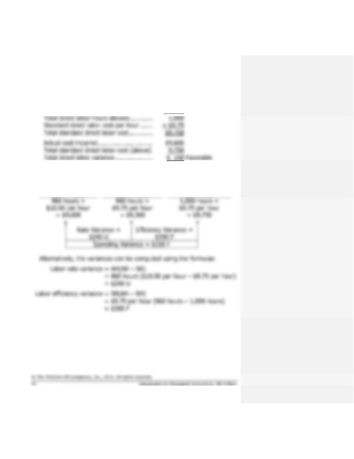
2.
Actual Hours of
Input, at the
Actual Rate
Actual Hours of Input,
at the Standard Rate
Standard Hours
Allowed for Output, at
the Standard Rate
(AH × AR)
(AH × SR)
(SH × SR)
$10.00 per hour
Exercise 8-6 (20 minutes)
1.
Number of items shipped …………………………...
120,000
Standard direct labor-hours per item …………….
× 0.02
2.
Actual Hours of
Input, at the
Actual Rate
Actual Hours of Input,
at the Standard Rate
Standard Hours
Allowed for Output, at
the Standard Rate
(AH × AR)
(AH × SR)
(SH × SR)
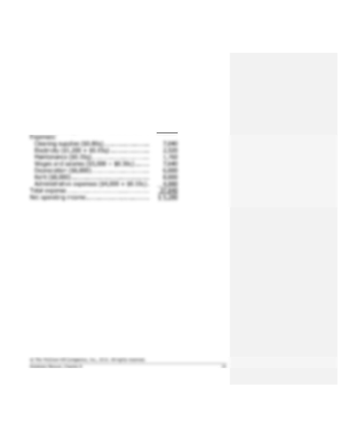
Exercise 8-7 (15 minutes)
Lavage Rapide
Planning Budget
For the Month Ended August 31
Budgeted cars washed (q) ………………………..
9,000
Revenue ($4.90q) …………………………..………
$44,100
Expenses:
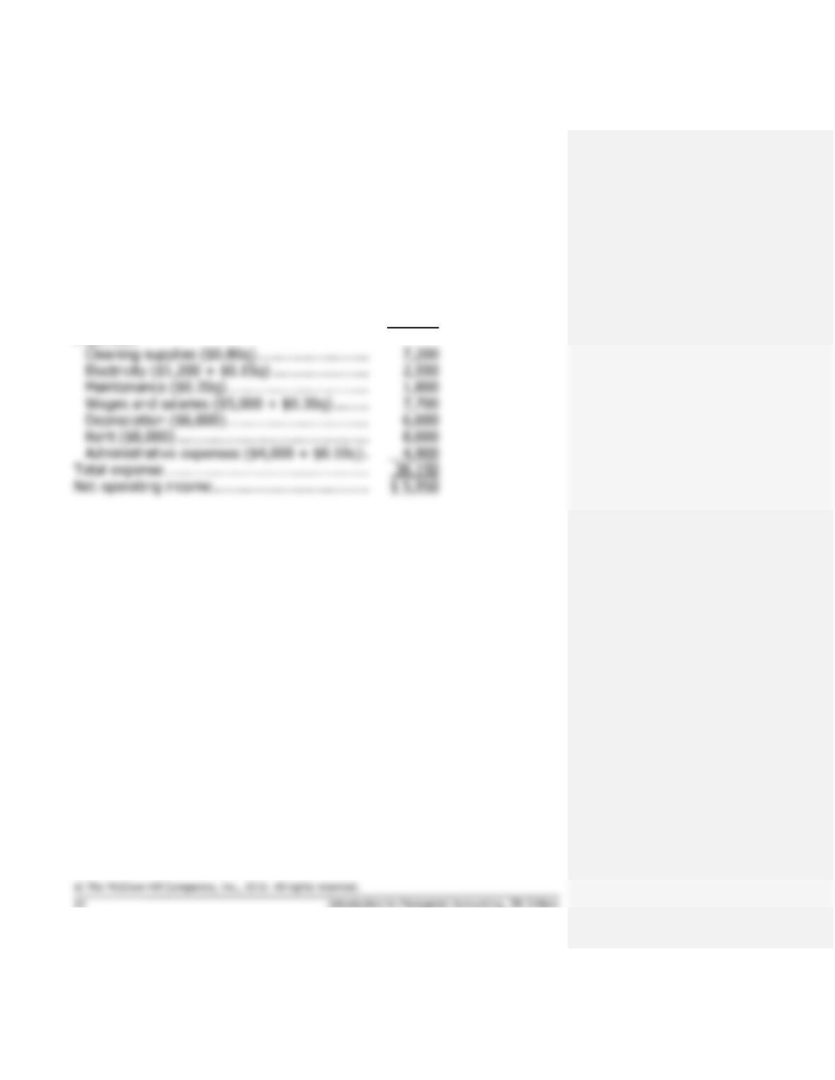
Exercise 8-8 (15 minutes)
Lavage Rapide
Flexible Budget
For the Month Ended August 31
Actual cars washed (q) …………………………….
8,800
Revenue ($4.90q) …………………………..………
$43,120
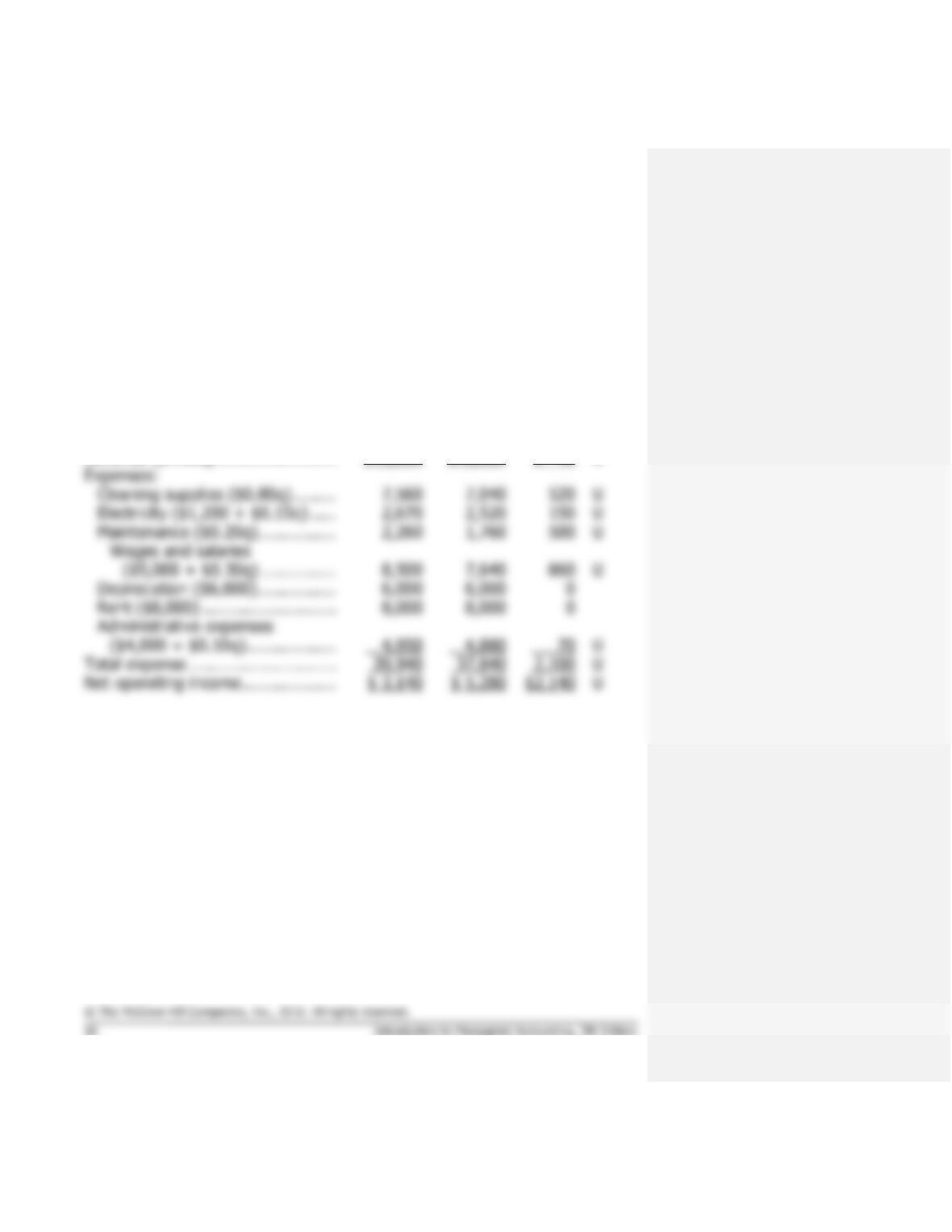
Exercise 8-9 (20 minutes)
Lavage Rapide
Revenue and Spending Variances
For the Month Ended August 31
Actual
Results
Flexible
Budget
Revenue
and
Spending
Variances
Cars washed (q) ……………………..
8,800
8,800
Revenue ($4.90q) ……………………
$43,080
$43,120
$ 40
U
Expenses:
8,000
8,000
Total expense …………………………
U
Net operating income ……………….
U
Exercise 8-10 (30 minutes)
1.
Number of units manufactured ………………………..
20,000
Standard labor time per unit
(18 minutes ÷ 60 minutes per hour) ………………
× 0.3
Total standard direct labor cost ……………………….
Actual direct labor cost ………………………………….
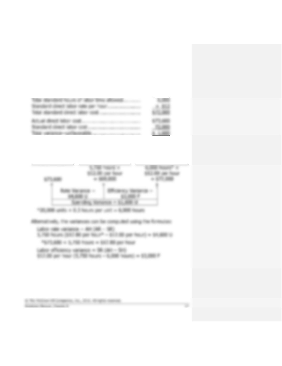
2.
Actual Hours of
Input, at the
Actual Rate
Actual Hours of Input,
at the Standard Rate
Standard Hours Allowed
for Output, at the
Standard Rate
(AH × AR)
(AH × SR)
(SH × SR)
$12.00 per hour
$12.00 per hour
= $69,000
= $72,000
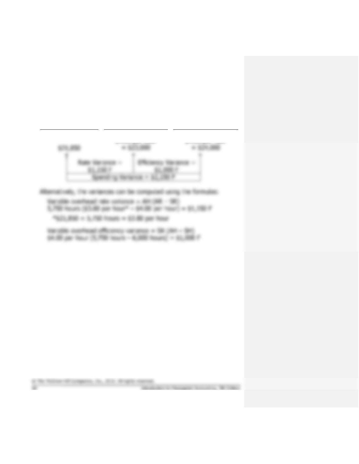
Exercise 8-10 (continued)
3.
Actual Hours of
Input, at the
Actual Rate
Actual Hours of Input,
at the Standard Rate
Standard Hours
Allowed for Output, at
the Standard Rate
(AH × AR)
(AH × SR)
(SH × SR)
5,750 hours ×
6,000 hours ×
Exercise 8-11 (20 minutes)
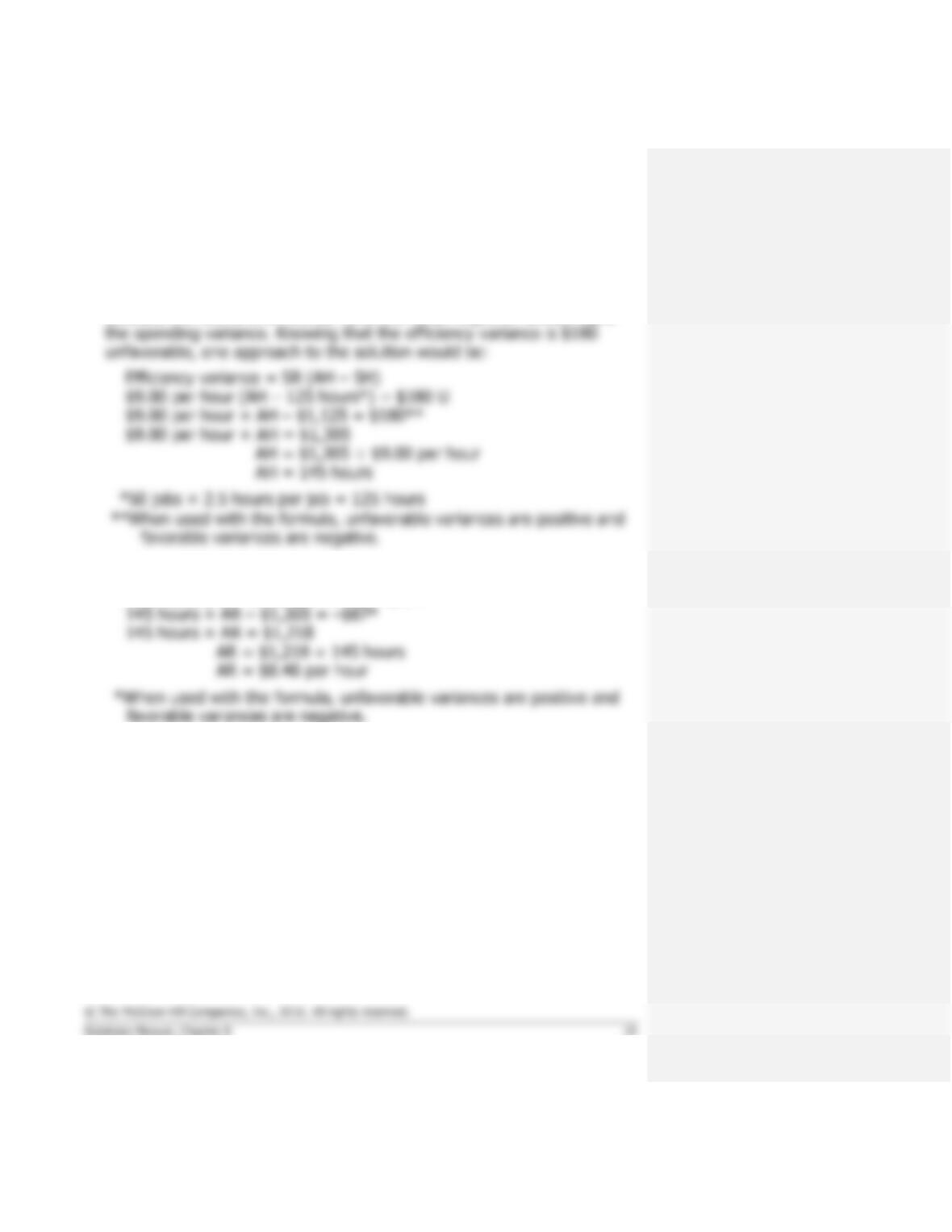
1. If the labor spending variance is $93 unfavorable, and the rate variance
is $87 favorable, then the efficiency variance must be $180 unfavorable,
because the rate and efficiency variances taken together always equal
2. Rate variance = AH (AR – SR)
145 hours (AR – $9.00 per hour) = $87 F
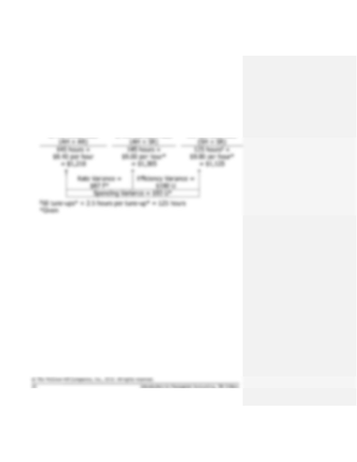
Exercise 8-11 (continued)
An alternative approach would be to work from known to unknown data
in the columnar model for variance analysis:
Actual Hours of Input,
at the Actual Rate
Actual Hours of Input,
at the Standard Rate
Standard Hours
Allowed for Output, at
the Standard Rate