CHAPTER 7/HYPOTHESIS TESTING: ONE SAMPLE INFERENCE 133
N Mean StDev SE Mean
Calor_dr 173 1619.9 323.4 24.6
7.66 After creating new variables representing percentage of calories from fat (saturated fat) for both DR and
FFQ, and performing two-sample t-tests as in 7.59, we get:
Paired T-Test and CI: TFpDR, TFpFFQ
Paired T for TFpDR – TFpFFQ
N Mean StDev SE Mean
Paired T-Test and CI: SFpDR, SFpFFQ
Paired T for SFpDR – SFpFFQ
N Mean StDev SE Mean
SFpDR 173 0.13804 0.02115 0.00161
7.67 Using the data set SEXRAT>DAT, and still assuming the overall probability of having a male child is
#children
total#
families
Expected
P(allmale)
Expected
P(allfemale)M(#allmale)CIF(#allfemale)CI
3122790.12960.1206 1651 (0.1284,0.1405)1498(0.1162,0.1278)
134 CHAPTER 7/HYPOTHESIS TESTING: ONE SAMPLE INFERENCE
7.68 For this solution, we will create the variables HDif and SDif, which refer to the difference between
baseline values of heart rate and SBP and the “Lv1” observations. Once we obtain summary statistics for
each treatment group, we get
Descriptive Statistics: HDif, SDif
Variable Trtgrp N N* Mean SE Mean
HDif N 18 0 6.11 2.51
7.69 We wish to test the hypothesis H00
37:.
P
P
vs. H10
:
P
P
z, where
P
true expected number of
events among subjects with 250 treatments. We will use the small sample version of the one sample
P
7.71 From Problem 7.69, there is no significant difference between observed melanoma rates among the group
P
7.72 We wish to test the hypothesis
H
pp
00
: vs. Hp p
10
: z, where p = true incidence rate of breast cancer
CHAPTER 7/HYPOTHESIS TESTING: ONE SAMPLE INFERENCE 135
7.74 The projected number of new cases of breast cancer from age 40 to age 70 in the general population
7.75 The principal advantage is that we are using each person as their own control. Since different people
7.76 There are 7 left eyes assigned to A and 3 left eyes assigned to P. If the assignments are really random,
7.77 A comparison of itching scores for the active-treated eye
XAi
vs. the placebo-treated eye
XPi
for the
ith subject is given by
d
X
X
i
A
i
P
i
.
136 CHAPTER 7/HYPOTHESIS TESTING: ONE SAMPLE INFERENCE
7.78 We compute di for each subject from Table 7.8 and 7.9 as follows:
i
X
Ai
X
Pi dii
X
Ai
X
Pi di
1 1 2 –1 6 2 3 –1
where
Hence,
One-Sample T: fnD
Test of mu = 0 vs not = 0
CHAPTER 7/HYPOTHESIS TESTING: ONE SAMPLE INFERENCE 137
7.80 For femoral shaft BMD, we again fail to reject the null hypothesis at the 0.05 level.
One-Sample T: fsD
7.82 We use the large sample method. We have a 95% CI for ln(μ) given by:
7.85 If the rate was .0315 events per person-year, we would expect .0315(9539.92) = 300.5 HIV cases,
7.86 This simulation can be performed in multiple programming languages, but we will show the code used in R:
138 CHAPTER 7/HYPOTHESIS TESTING: ONE SAMPLE INFERENCE
7.88 We can easily change the rnorm() command to generate random normal data with a mean of 115; after
7.89 We found a significant result in 62% of our samples. To determine the rate for a large number of
simulated samples, we can use the power formula:
7.90 We wish to test the hypothesis 0010
:vs.:
H
pp Hpp z, where 0
p= incidence rate of neuroblastoma
in the general population 5
7.3 10 and p = incidence rate of neuroblastoma in the screened population.
7.91 A 95% CI for p is given by ˆˆˆ
1.96ppqnr. In this case,
45
ˆ204 1, 475, 773 1.38 10 13.8 10p
u
CHAPTER 7/HYPOTHESIS TESTING: ONE SAMPLE INFERENCE 139
7.92 We wish to test the hypothesis 01
:16vs.:16Hp Hp z. We have that
00 204 1 6 5 6 28.3 5np q t
. Thus, we can use the normal approximation to the binomial. We
have the test statistic
7.93 We wish to test the hypothesis 0010
:vs.:
H
pp Hpp z, where
7.94 The test statistic is
7.95 In this case,
ˆˆ 586 11 586 575 586 10.8 5npq t
.
140 CHAPTER 7/HYPOTHESIS TESTING: ONE SAMPLE INFERENCE
7.96 For these exercises, we have 4 measurements taken at each time point (2 measurements per eye), so our
7.97 Comparing the 5, 10, and 15-minute measurements to the “immediate” measurements, we find that
One-Sample T: ImChange5, ImChange10, ImChange15
Test of mu = 0 vs not = 0
7.99 We wish to compute
P
We will approximate X by a normal distribution Y with mean = variance = 42.
Hence,
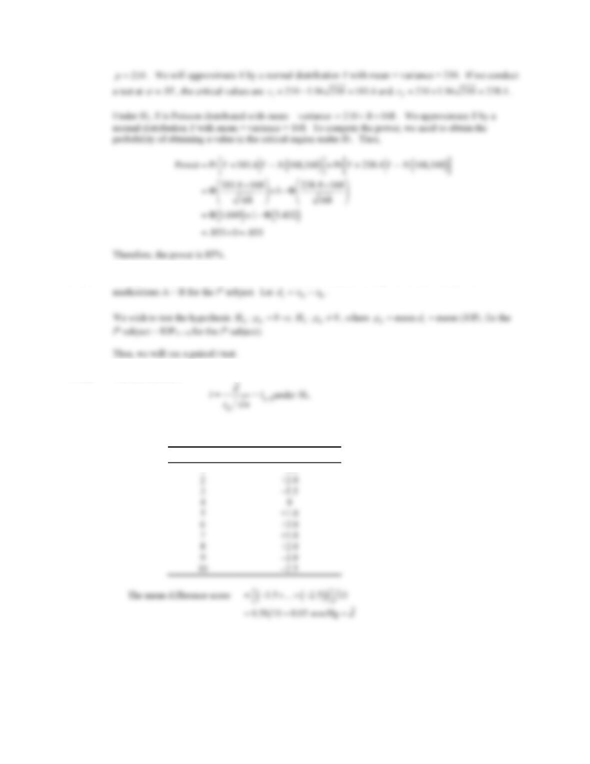
7.100 If 10 medical residents participate for a 3 week period, then 10 21 210
P
u . We will use the normal
approximation to the Poisson distribution. Under H0, the number of errors (X) is Poisson distributed with
CHAPTER 7/HYPOTHESIS TESTING: ONE SAMPLE INFERENCE 141
7.101 Let
2IOP
i
x after 60 days on medication C for the ith subject. Let 1IOP
i
x after 60 days on
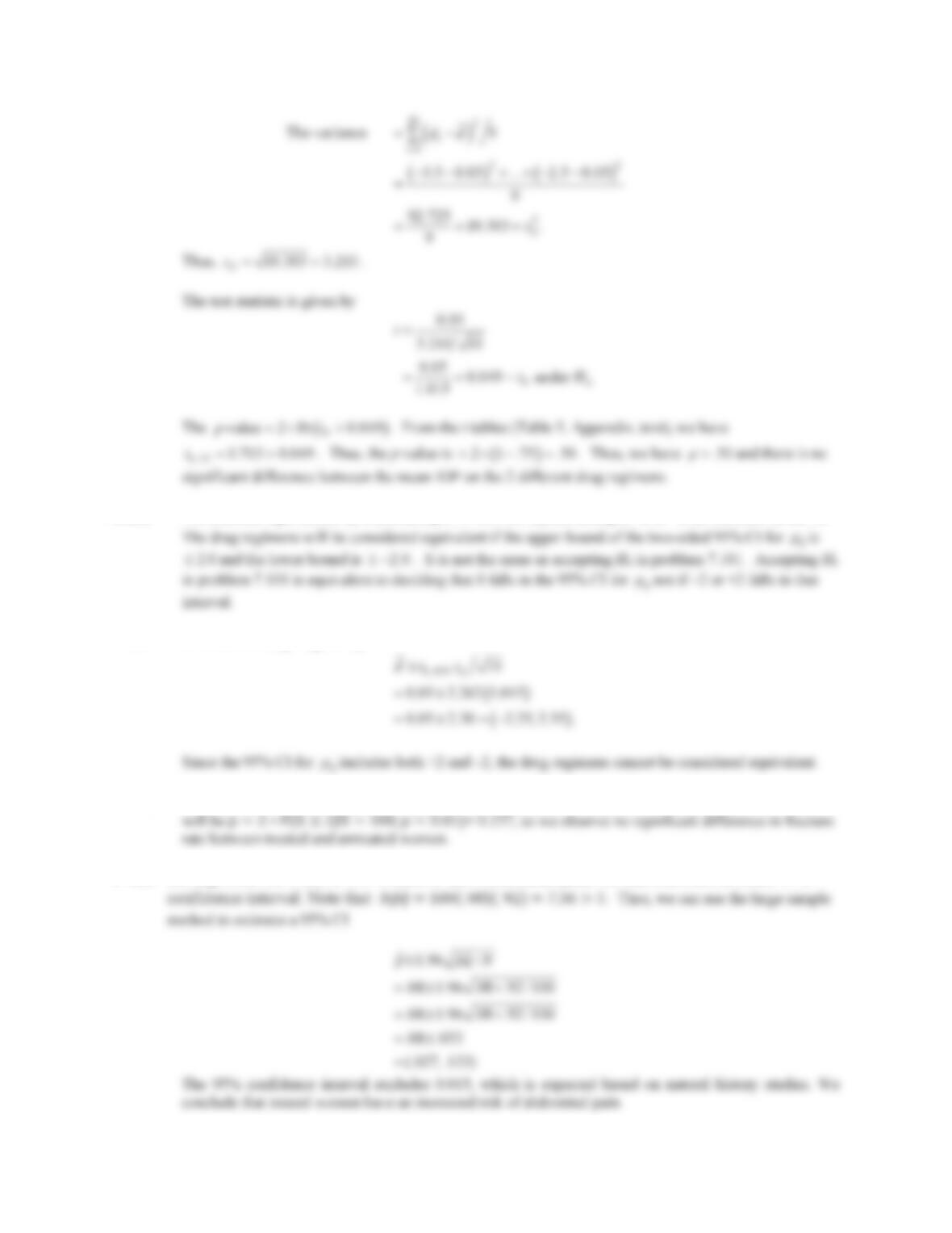
7.102 The test statistic is
We have the following difference scores
Subject #(i) 21iii
dx x
142 CHAPTER 7/HYPOTHESIS TESTING: ONE SAMPLE INFERENCE
7.103 We establish equivalence by constructing a 95% CI for d
P
and noting if +2 or –2 are included in the CI.
P
P
7.104 A 95% CI for d
P
is given by
P
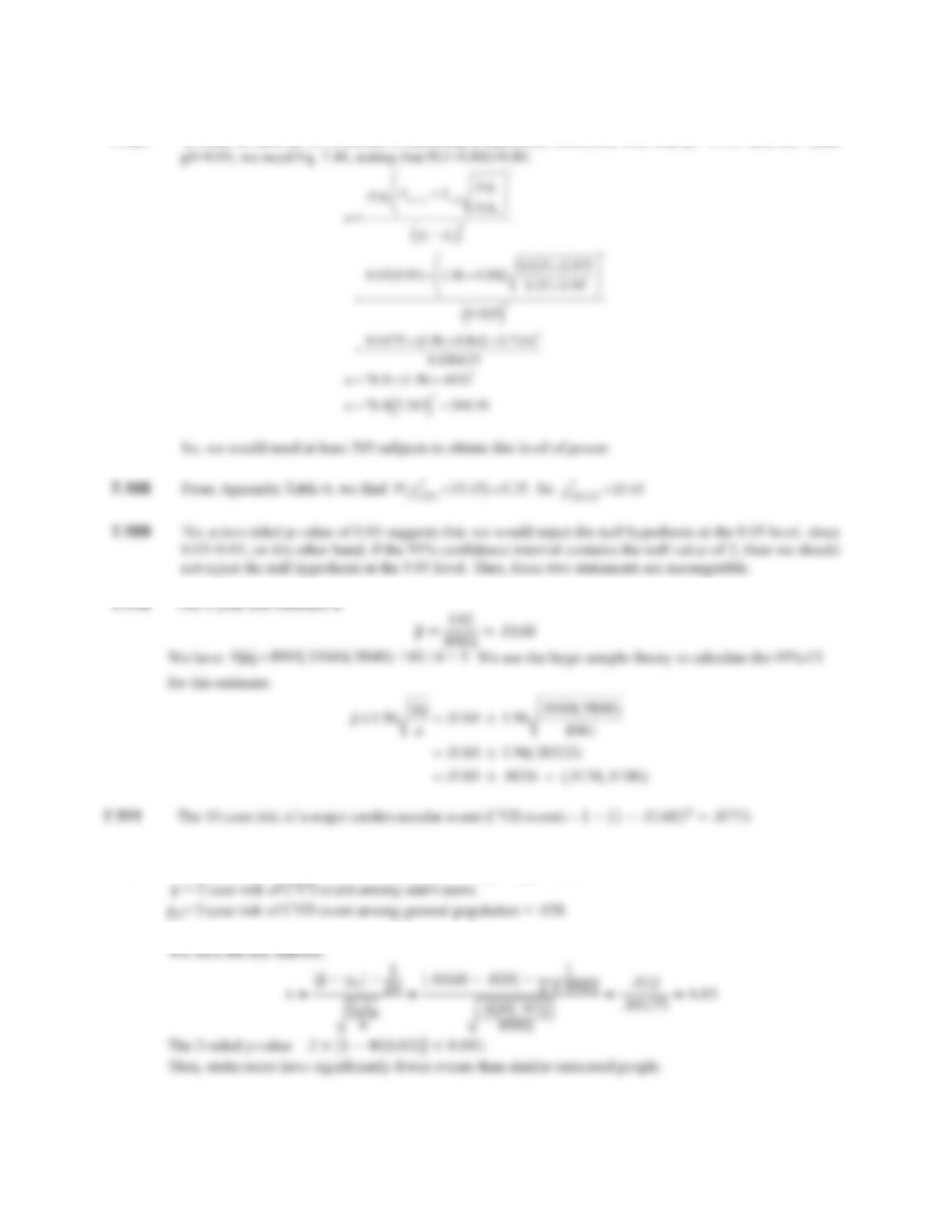
7.105 We wish to test the null hypothesis ܪǣൌͲǤͲͷvs ܪଵǣ്ͲǤͲͷǤ The two-tailed p-value for this test
7.106Having observed 8 out of 100 women to have abdominal pain, we can construct an exact 95%
CHAPTER 7/HYPOTHESIS TESTING: ONE SAMPLE INFERENCE 143
7.107 In order to have an 80% chance of detecting a significant difference with true p1=0.025 and null value
7.112 We wish to test the hypotheses: ǣൌ vs. ଵǣ് where:
7.113 The expected event rate based on LDL reduction is:
144 CHAPTER 7/HYPOTHESIS TESTING: ONE SAMPLE INFERENCE
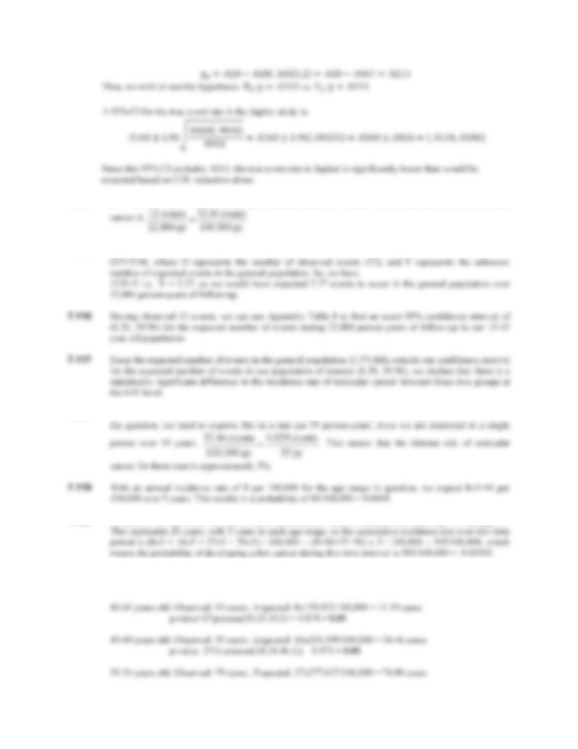
7.114 If we observe 12 events in 22,884 person-years, then our estimate of the incidence rate for testicular
7.115 If 12 events out of 22,884 person-years represents a standardized incidence rate of 5.06, then we have
7.118 In 7.112, we estimated the risk in this population to be 52.44 events per 100,000 person-years. To answer
7.120 To answer this question, we need to sum the incidence rates for each year between age 40 and age 59.
7.121 We will evaluate each age group separately, using the exact confidence interval for the first two age
groups, and a normal approximation for the latter two groups.
CHAPTER 7/HYPOTHESIS TESTING: ONE SAMPLE INFERENCE 145