
7-1
CHAPTER 7
ALLOCATING COSTS OF SUPPORT DEPARTMENTS
AND JOINT PRODUCTS
DISCUSSION QUESTIONS
1. Stage one assigns service costs to produc-
ing departments. Costs are assigned using
factors that reflect the consumption of the
services by each producing department.
Stage two allocates the costs assigned to
the producing departments (including ser-
vice costs and direct costs) to the products
passing through the producing departments.
2. GAAP requires that all manufacturing costs
be assigned to products for inventory valua-
tion.
3. Allocation of service costs aids in planning be-
cause it makes users pay attention to the level
of service activity being consumed and also
provides an incentive for them to monitor the
efficiency of the service departments. It aids in
pricing because support department costs are
part of the cost of producing a product. Know-
ing the individual product costs is helpful for
developing bids and cost–plus prices.
4. Without any allocation of service costs, us-
ers may view services as a free good and
consume more of the service than is opti-
mal. Allocating service costs would encour-
age managers to use the service until such
time as the marginal cost of the service is
equal to the marginal benefit.
5. Since the user departments are charged for
the services provided, they will monitor the
performance of the service department. If the
service can be obtained more cheaply exter-
nally, then the user departments will be likely
to point this out to management. Knowing
this, a manager of a service department will
exert effort to maintain a competitive level of
service.
6. The identification and use of causal factors
ensures that service costs are accurately
assigned to users. This increases the legiti-
macy of the control function and enhances
product costing accuracy.
7. Allocating actual costs passes on the effi-
ciencies or inefficiencies of the service de-
partment, something that the manager of the
producing department cannot control. Allo-
cating budgeted costs avoids this problem.
8. Variable costs should be allocated according
to usage, whereas fixed costs should be al-
located according to capacity. Variable costs
are based on usage because, as a depart-
ment’s usage of a service increases, the
variable costs of the service department in-
crease. A service department’s capacity and
the associated fixed costs were originally set
by the user departments’ capacities to use
the service. Thus, each department should
receive its share of fixed costs as originally
conceived (to do otherwise allows one de-
partment’s performance to affect the amount
of cost assigned to another department).
9. Normal or peak capacity measures the orig-
inal capacity requirements of each produc-
ing department. It is used when one
department’s spike in usage affects the
amount of capacity needed.
10. Using variable bases to allocate fixed costs
allows one department’s performance to af-
fect the costs allocated to other depart-
ments. Variable bases also fail to reflect the
original consumption levels that essentially
caused the level of fixed costs.
11. The dual-rate method separates the fixed and
variable costs of providing services and
charges them separately. In effect, a single
rate treats all service costs as variable. This
can give faulty signals regarding the marginal
cost of the service. If all costs of the service
department were variable, there would be no
need for a dual rate. In addition, if original ca-
pacity equaled actual usage, the dual-rate
method and the single-rate method would
give the same allocation.
12. The direct method allocates the direct costs of
each service department directly to the
producing departments. No consideration is
given to the fact that other service centers
may use services. The sequential method
allocates service costs sequentially. First, the

7-2
costs of the center providing the greatest
service are allocated to all user departments,
including other service departments. Next, the
costs of the second greatest provider of
services are allocated to all user departments,
excluding any department(s) that have
already allocated costs. This continues until
all service center costs have been allocated.
The principal difference in the two methods is
the fact that the sequential method considers
some interactions among service centers and
the direct method ignores interactions.
13. The reciprocal method is more accurate be-
cause it fully considers interactions among
service centers.
14. A joint cost is a cost incurred in the simulta-
neous production of two or more products.
At least one of these joint products must be
a main product. It is possible for the joint
production process to produce a product of
relatively little sales value relative to the
main product(s); this product is known as a
by-product.
15. Joint costs occur only in cases of joint pro-
duction. A joint cost is a common cost, but a
common cost is not necessarily a joint cost.
Many overhead costs are common to the
products manufactured in a factory but do
not signify a joint production process.
7-3
CORNERSTONE EXERCISES
Cornerstone Exercise 7.1
1. Total expected costs of the Maintenance Department:
Fixed costs …………………………………………………………………………… $64,900
2. Charge based on actual usage = Charging rate × Actual maintenance hours
Assembly Department charge = $4.30 × 3,960 = $17,028
3. Assembly Department charge = $4.30 × 4,000 = $17,200
Cornerstone Exercise 7.2
1. Variable rate = $1.35 per maintenance hour
The fixed allocation is calculated for each department based on budgeted
peak month usage:
Peak Number Budgeted Allocated
Department of Hours Percent* Fixed Cost Fixed Cost
Assembly……………….. 390 15% $64,900 $ 9,735
7-4
Cornerstone Exercise 7.2 (continued)
Percent for Fabricating = 1,300/2,600 = 0.50, or 50%
2. Actual Number Variable Variable Fixed Total
Department of Hours Rate Amount Amount Charge
3. Actual Number Variable Variable Fixed Total
Department of Hours Rate Amount Amount Charge
Assembly …… 4,000 $1.35 $ 5,400 $ 9,735 $15,135
7-5
Cornerstone Exercise 7.3
1. Allocation ratios:
Proportion of Driver Used by
Human General
Resources Factory Fabricating Assembly
Human Resources — — 0.321 0.682
General Factory — — 0.303 0.704
2. Support Departments Producing Departments
Human General
Resources Factory Fabricating Assembly
Direct costs $ 160,000 $ 340,000 $114,600 $ 93,000
3. Since none of the Human Resources cost is allocated to General Factory, it
7-6
Cornerstone Exercise 7.4
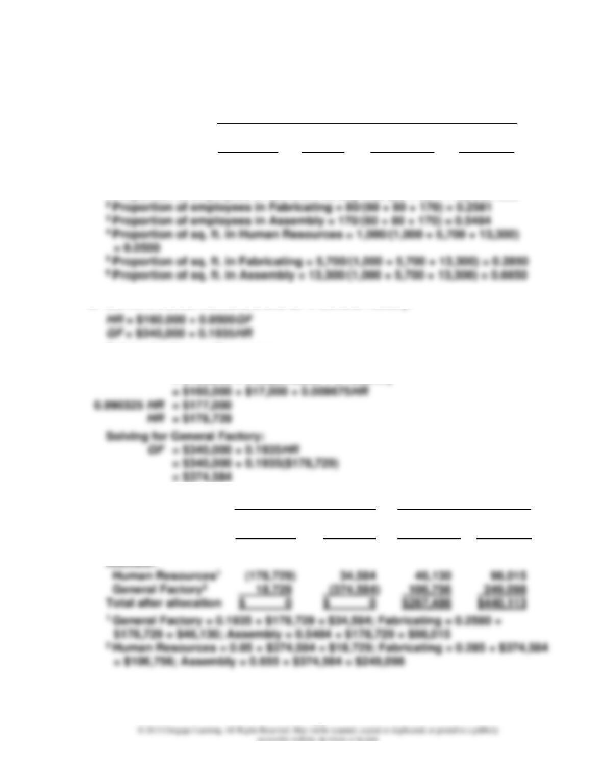
1. Allocation ratios with General Factory ranked first:
Proportion of Driver Used by
Human General
Resources Factory Fabricating Assembly
Human Resources — — 0.32001 0.68002
General Factory 0.05003 — 0.28504 0.66505
2. Support Departments Producing Departments
Human General
Resources Factory Fabricating Assembly
Direct costs $ 160,000 $ 340,000 $114,600 $ 93,000
Allocate:
3. Typically, rounding the allocation ratios to six significant digits would produce
7-7
Cornerstone Exercise 7.5
1. Allocation ratios:
Proportion of Driver Used by
Human General
Resources Factory Fabricating Assembly
Human Resources — 0.19351 0.25812 0.54843
General Factory 0.05004 — 0.28505 0.66506
1 Proportion of employees in General Factory = 60/(60 + 80 + 170) = 0.1935
2. Let HR = Human Resources and GF = General Factory.
Solving for Human Resources:
HR = $160,000 + 0.05GF
= $160,000 + 0.05($340,000 + 0.1935HR)
3. Support Departments Producing Departments
Human General
Resources Factory Fabricating Assembly
Direct costs $ 160,000 $ 340,000 $114,600 $ 93,000
4. If Fabricating had the bulk of the square footage, it would get the largest allo-
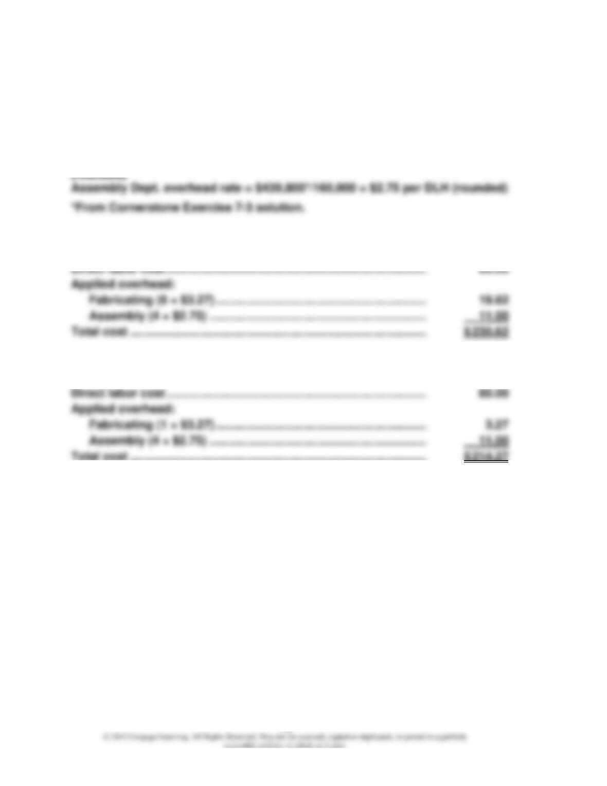
7-8
cation of General Factory costs. As a result, Fabricating would have the major-
ity of support department costs, instead of Assembly.
Cornerstone Exercise 7.6
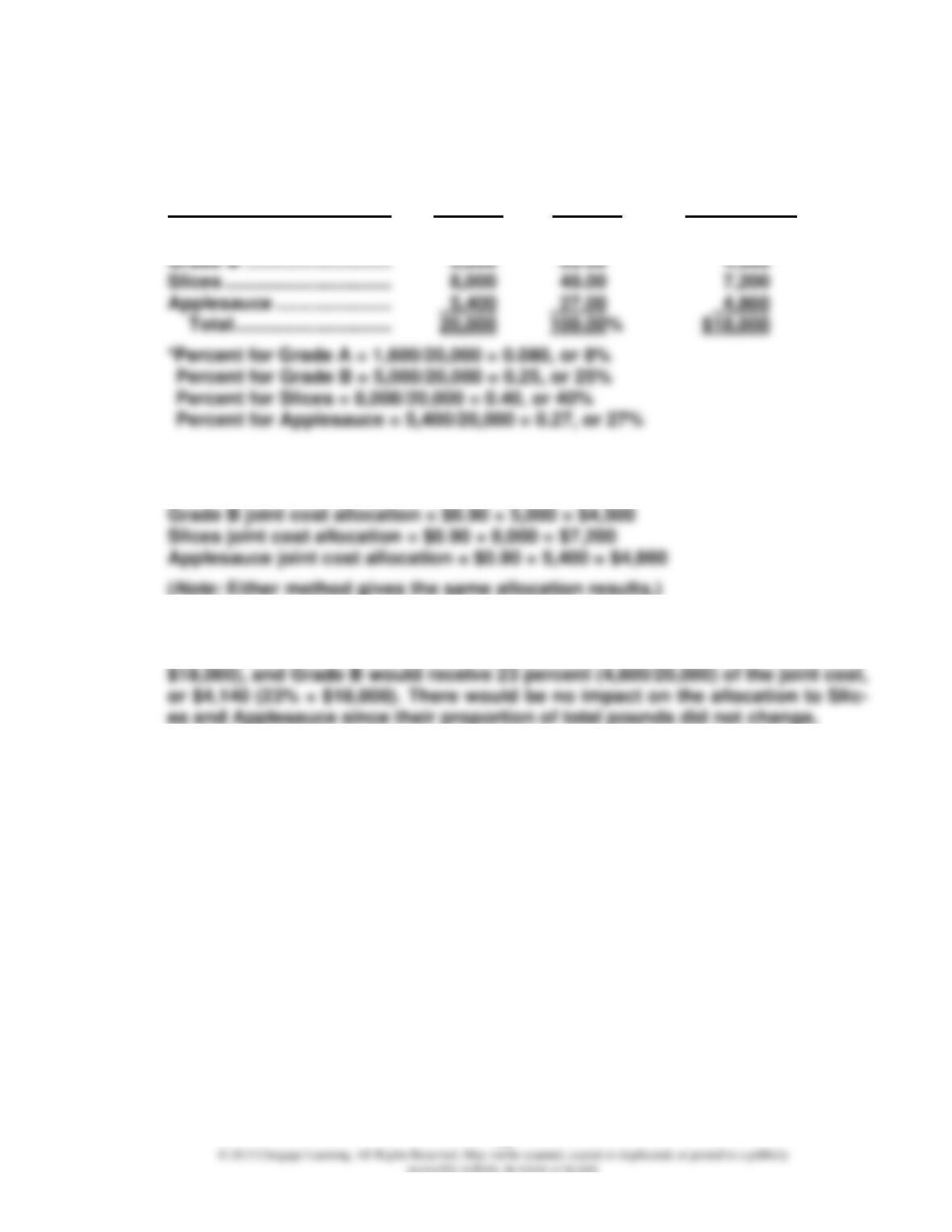
1. Fabricating Dept. overhead rate = $267,800*/82,000 = $3.27 per mach. hr.
2. Cost of Job 316:
Direct materials …………………………..……………………………………….. $ 120.00
3. New Cost of Job 316:
Direct materials …………………………..……………………………………….. $ 120.00
7-9
Cornerstone Exercise 7.7
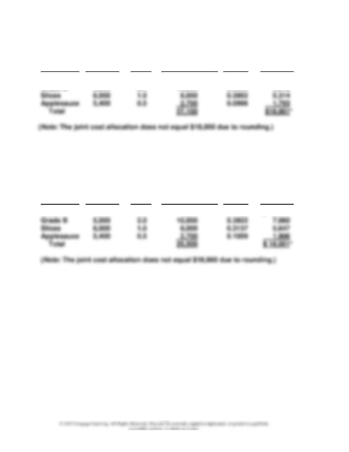
1. Percent Joint Cost
Pounds of Units* Allocation
Grades (2) (3) (3) × $18,000
Grade A ………………………. 1,600 8.00% $ 1,440
2. Average joint cost = $18,000/20,000 pounds = $0.90 per pound
Grade A joint cost allocation = $0.90 × 1,600 = $1,440
3. If Grade A had 2,000 pounds and Grade B had 4,600 pounds, then Grade A
would receive 10 percent (2,000/20,000) of the joint cost, or $1,800 (10% ×
7-10
Cornerstone Exercise 7.8
1. Number Weight Weighted Number Allocated
Grades of Pounds Factor of Pounds Percent Joint Cost
Grade A 1,600 4.0 6,400 0.2362 $ 4,252
Grade B 5,000 2.0 10,000 0.3690 6,642
2. If the Grade A weight factor is decreased to 3.0, then the weighted number of
pounds would decrease by one-fourth and the Grade A apples would receive a
relatively smaller amount of joint cost. However, the allocation of cost to all
other grades will increase since the decreased weighted pounds for Grade A
apples will impact all percentages. The following table shows what would
happen:
Number Weight Weighted Number Allocated
Grades of Pounds Factor of Pounds Percent Joint Cost
Grade A 1,600 3.0 4,800 0.1882 $ 3,388
7-11
Cornerstone Exercise 7.9
1.
Price at Total Market Percent Allocated
Pounds Split-Off Value at of Total Joint
Grades Produced (per pound) Split-Off Market Value Cost
Grade A 1,600 $4.00 $ 6,400 0.4015 $ 7,227
2. If the price of Grade B apples increases to $1.20 per pound, then Grade B
would have a higher market value and would receive a higher percentage of
joint cost. The other three grades would have somewhat lower joint cost allo-
cations. Results of this change follow:
Price at Total Market Percent Allocated
Pounds Split-Off Value at of Total Joint
Grades Produced (per pound) Split-Off Market Value Cost
Grade A 1,600 $4.00 $ 6,400 0.3778 $ 6,800
Grade B 5,000 1.20 6,000 0.3542 6,376
7-12
Cornerstone Exercise 7.10
1.
Further Hypothetical Hypothetical Allocated
Market Processing Market Number Market Joint
Product Price Cost Price of Gallons Value Percent* Cost**
(1) – (2) = (3) × (4) = (5)
L-Ten $2.00 $0.50 $1.50 3,500 $ 5,250 0.1615 $ 2,083
Pioze 6.00 1.50 4.50 2,500 11,250 0.3462 4,466
Total $ 32,500 $ 12,900
*Percent for L-Ten = $5,250/$32,500 = 0.1615, or 16.15%
Percent for Triol = $16,000/$32,500 = 0.4923, or 49.23%
2. If it cost $2 to process each gallon of Triol, the hypothetical market price
would be less, the hypothetical market value would be less, and Triol would
receive a smaller allocation of joint cost. The following table shows the re-
sults:
Further Hypothetical Hypothetical Allocated
Market Processing Market Number Market Joint
Product Price Cost Price of Gallons Value Percent* Cost**
(1) – (2) = (3) × (4) = (5)
L-Ten $2.00 $0.50 $1.50 3,500 $ 5,250 0.1842 $ 2,376
Triol 5.00 2.00 3.00 4,000 12,000 0.4211 5,432
*Percent for L-Ten = $5,250/$28,500 = 0.1842, or 18.42%
Percent for Triol = $12,000/$28,500 = 0.4211, or 42.11%
7-13
Cornerstone Exercise 7.11
1. Total revenue:
L-Ten ($2 × 3,500) …………………………..……………… $ 7,000
Further processing costs:
L-Ten ($0.50 × 3,500) ……………………………………… $ 1,750
2. Gross margin percentage = Gross margin/Total revenue
= $19,600/$42,000 = 0.4667, or 46.67% (rounded)
L-Ten Triol Pioze
Eventual market value …………………. $7,000 $ 20,000 $ 15,000
Less: Gross margin at 46.67% ……… 3,267 9,334 7,001
is $12,898.)
3. An increase in the further processing cost of Triol will reduce the gross mar-
gin percentage and will decrease the joint cost allocated to Triol.
Total revenue ……………………………………………………………………….. $ 42,000
Further processing costs ……………………………………………………… (13,500)
L-Ten Triol Pioze
Eventual market value …………………. $7,000 $ 20,000 $ 15,000
Less: Gross margin at 37.14% ……… 2,600 7,428 5,571
EXERCISES
Exercise 7.12
a. support f. support k. support
Exercise 7.13
a. support e. producing i. producing
Exercise 7.14
a. Number of employees
b. Square footage
7-15
Exercise 7.15
1. Dr. Poston may want to cost the cleanser for several reasons: to value inven-
tory, to determine profitability, and to plan sales and costs for the coming
2. The situation has changed dramatically. Now, the cleanser should be allocat-
ed some of the office rent as well as all of the new assistant’s salary. The of-
fice rent could be apportioned 75 percent to the three doctors and 25 percent
to the cleanser bottling operation given that the cleanser operation takes an
office and an examining room. It could be argued that this overstates the al-
location to the cleanser, since the waiting room area does not serve the
Exercise 7.16
1. The incremental method of allocating the cost of the trip would result in a
2. The benefits-received approach could result in the following cost allocation
to Kallie:
Motel [$580 + ($15 × 4)]/3] …………. $ 213.33
7-16
Exercise 7.17
1. Single charging rate = [($1,800 + $1,500)/1,000*] + $1.20
Number Charging
Store of Gifts × Rate = Total
The Stationery Station ……………… 160 $4.50 $ 720
Arts & Collectibles ……………………. 420 4.50 1,890
Kid-Sports ……………………………….. 240 4.50 1,080
2. Number Allocated
Store of Gifts Percent Fixed Amount*
The Stationery Station ……………… 175 17.50% $ 577.50
Arts & Collectibles ……………………. 400 40.00 1,320.00
Kid-Sports ……………………………….. 100 10.00 330.00
Variable rate = $1.20 per gift
Number Variable Fixed Total
Store of Gifts Amount + Amount = Charge
The Stationery Station ……… 160 $ 192 $ 577.50 $ 769.50
Arts & Collectibles ……………. 420 504 1,320.00 1,824.00
Kid-Sports ……………………….. 240 288 330.00 618.00
7-17
Exercise 7.17 (Concluded)
3. The shops that actually use the gift-wrapping service less than anticipated
would like the single charging rate. The single charging rate assigns less of
the fixed cost to the shops using less of the service. Java Jim’s originally an-
4. Despite the charging rate method, Jeff may be overcharging by overestimat-
ing his fixed costs. The space used by the gift-wrapping service is one of
Exercise 7.18
1. Allocation ratios:
Year 1 Year 2
Department A ………. 0.4 0.5
Department B ………. 0.6 0.5
2. The manager of Department B is not controlling human resource costs better
3. First, variable and fixed costs should be allocated separately. Second, budg-
eted (not actual) costs should be allocated. Variable costs should be as-
Exercise 7.19
1. Product costing (Year 1 and Year 2 are identical):
Department A Department B
Variable costs:
($0.25 × 20,000) … $ 5,000
(0.5 × $100,000) … 50,000
2. Performance evaluation:
Year 1
Department A Department B
Variable costs:
($0.25 × 24,000) … $ 6,000
(0.5 × $100,000) … 50,000
(0.5 × $100,000) … 50,000
Total cost ………………. $56,000 $ 59,000
Year 2
Department A Department B
Variable costs:
($0.25 × 25,000) … $ 6,250
Fixed costs:
(0.5 × $100,000) … 50,000