106 CHAPTER 6/ESTIMATION
Therefore, the 95% CI for the variance is
6.66 We can estimate p directly from the sample proportion of people with latency time
6.67
Descriptive Statistics: Iqv
Total
Variable Lead_type Count Mean SE Mean StDev
Iqv 1 78 85.14 1.66 14.69
t8
CHAPTER 6/ESTIMATION 107
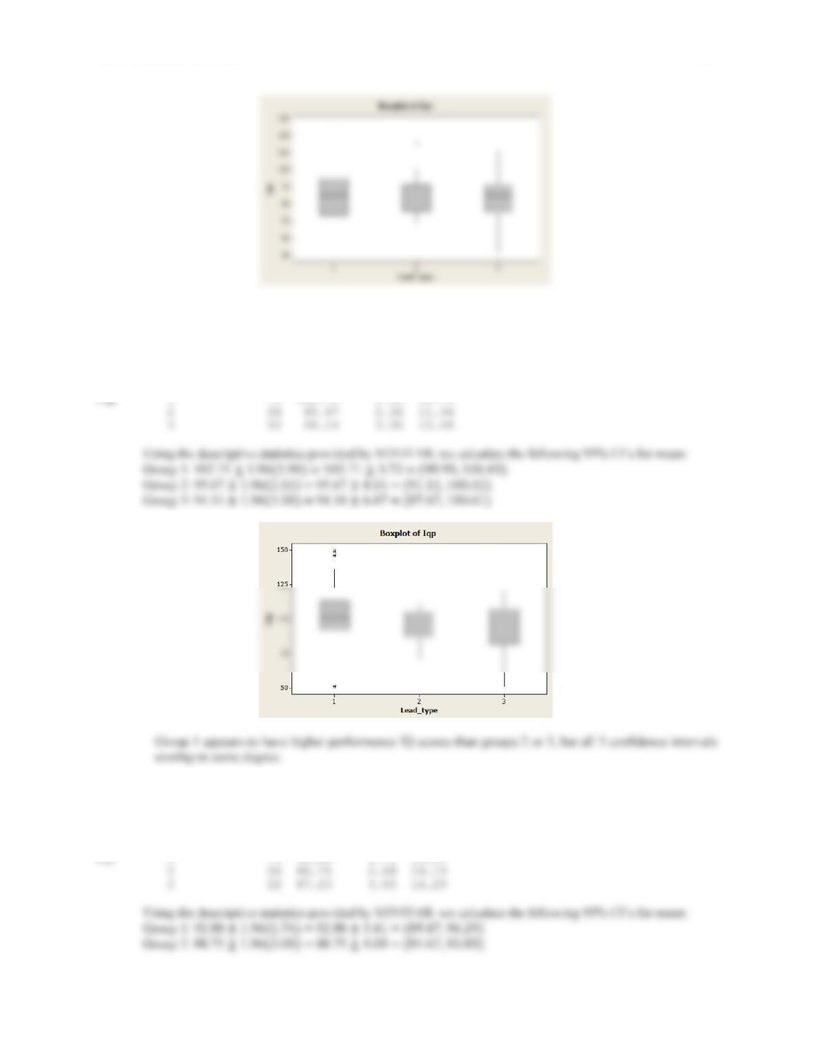
There is no obvious difference in verbal IQ scores by Lead Group.
6.68
Descriptive Statistics: Iqp
Total
Variable Lead_type Count Mean SE Mean StDev
Iqp 1 78 102.71 1.90 16.79
6.69
Descriptive Statistics: Iqf
Total
Variable Lead_type Count Mean SE Mean StDev
Iqf 1 78 92.88 1.74 15.34
108 CHAPTER 6/ESTIMATION
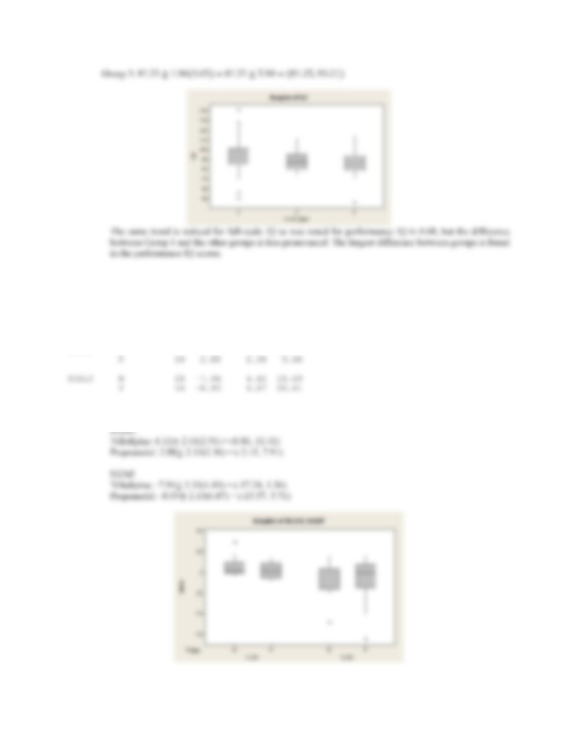
6.70 After creating variables “H1Dif” and “S1Dif”, representing change from baseline to Level 1 in heart rate
and SBP, respectively, we obtain the following summary statistics:
Descriptive Statistics: H1Dif, S1Dif
Total
Variable Trtgrp Count Mean SE Mean StDev
H1Dif N 18 6.11 2.51 10.67
The t-score needed for t(17) and t(15) distributions are 2.11 and 2.13, respectively
Our 95% CI’s are then:
CHAPTER 6/ESTIMATION 109
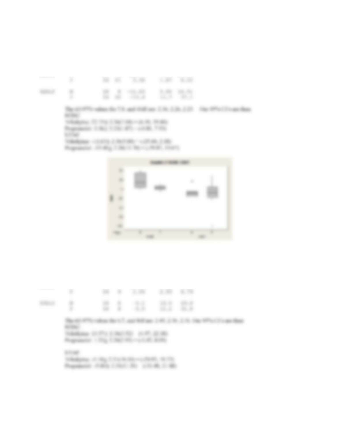
6.71 Again, after creating variables “H2Dif” and “S2Dif”, we note that there are several patients with missing
values, and get the following results:
Descriptive Statistics: H2Dif, S2Dif
Variable Trtgrp Count N Mean SE Mean StDev
H2Dif N 18 8 22.75 7.04 19.91
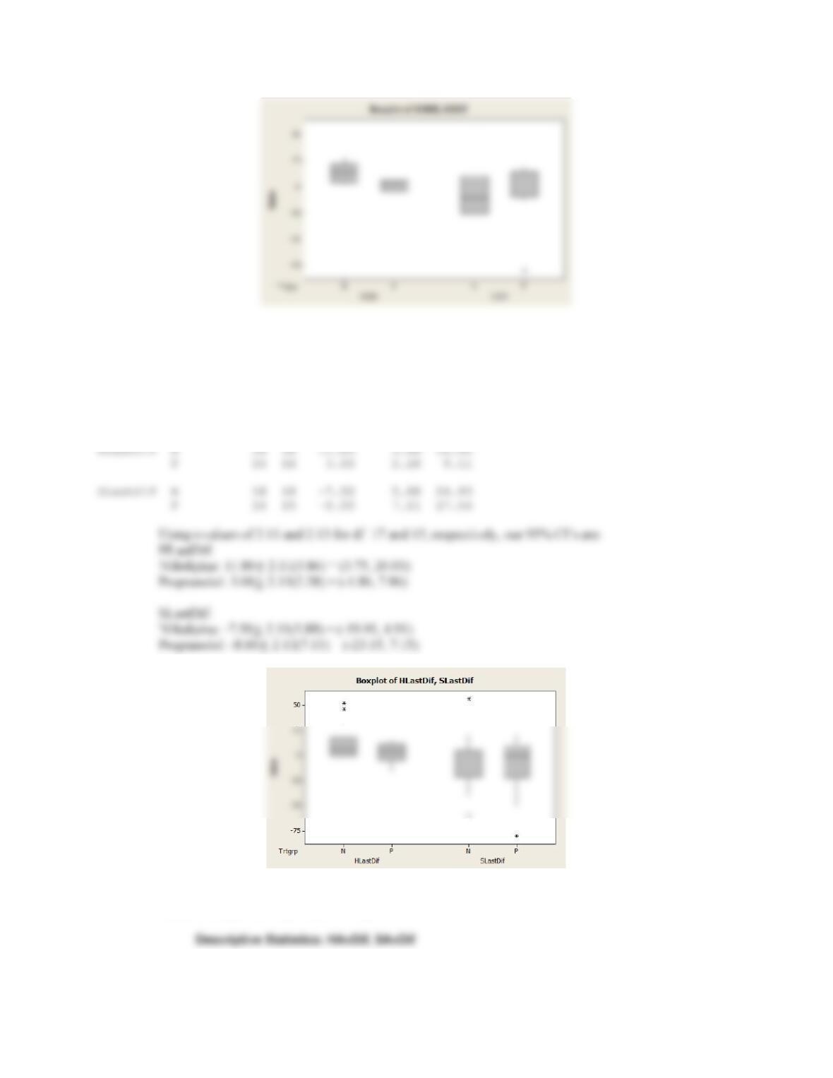
6.72 Repeating the procedure for “H3Dif” and “S3Dif”, we get the following:
Descriptive Statistics: H3Dif, S3Dif
Total
Variable Trtgrp Count N Mean SE Mean StDev
H3Dif N 18 7 13.57 3.52 9.31
110 CHAPTER 6/ESTIMATION
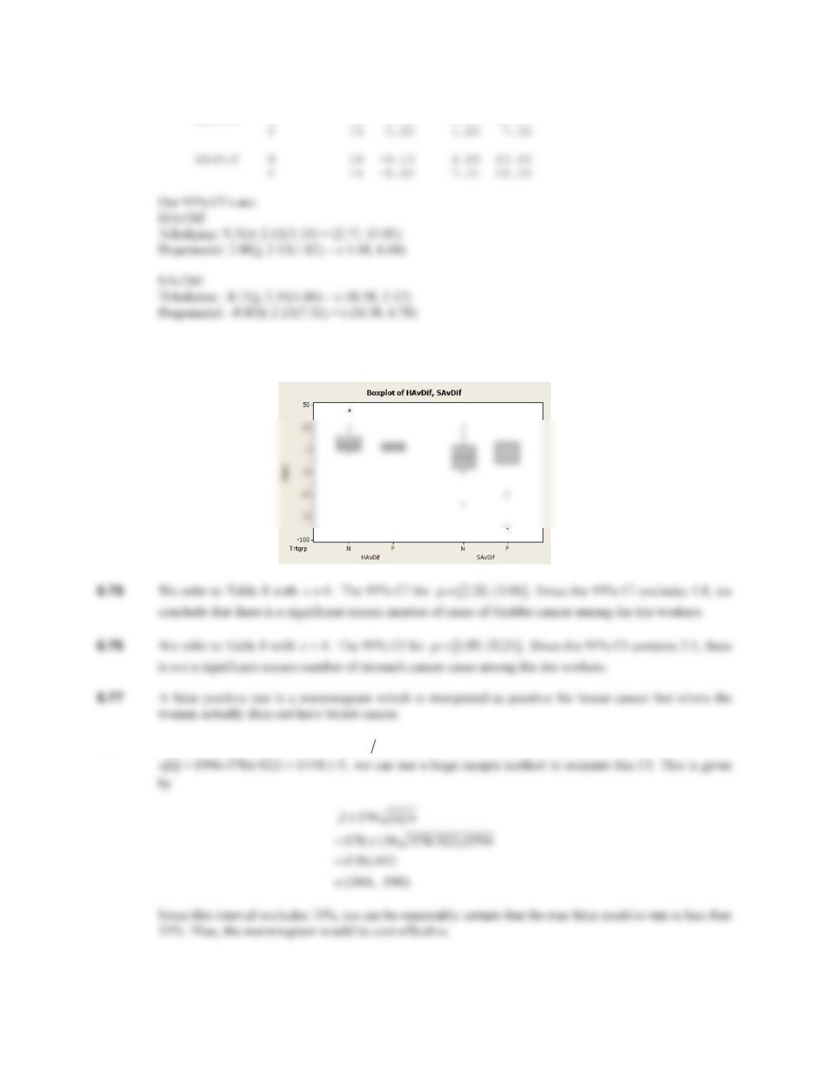
6.73 After creating “HLastDif” and “SLastDif”, we get:
Descriptive Statistics: HLastDif, SLastDif
Total
Variable Trtgrp Count N Mean SE Mean StDev
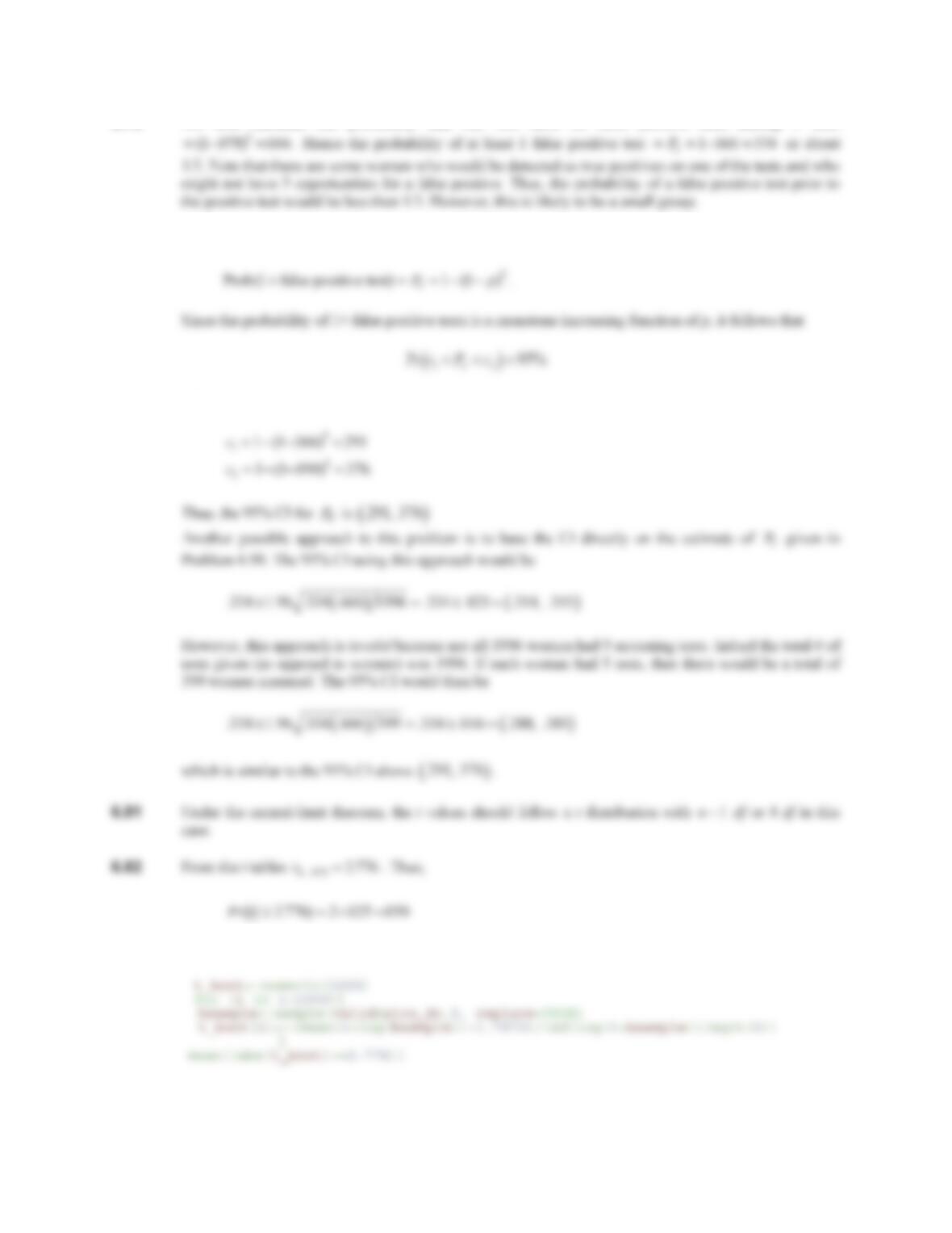
6.74 We can use the Calc Æ Row Statistics command to create HAv and SAv, and then subtract the baseline
values to create “HAvDif” and “SAvDif”:
Total
CHAPTER 6/ESTIMATION 111
Variable Trtgrp Count Mean SE Mean StDev
HAvDif N 18 9.31 3.10 13.17
Overall, there appears to be an mean increase in heart rate for the nifedipine group and comparable large
decreases in systolic blood pressure for both groups.
6.78 The estimated false positive rate . We will construct a 2-sided 95% CI for p. Since
156 1996 078.
p
112 CHAPTER 6/ESTIMATION
6.79 We first calculate the probability that she will have no false positive tests among 5 tests
6.80 From Problem 6.89, we know that . From Problem 6.79, we know that
where
6.83 We use the following R code to determine the percentage of t-values that exceeds 2.776 in absolute value
Pr . .066 090 95%
p
CHAPTER 6/ESTIMATION 113
P
6.85 A lower one-sided 90% CI for if the observed value is given by
6.86 First we create variable ‘fnD’=fn1-fn2. Descriptive statistics from MINITAB are shown:
Descriptive Statistics: fnD
6.87 Using the same procedure as in 6.86, we get the following results for the new variable ‘fsD’ = fs1-fs2
Descriptive Statistics: fsD
6.88 After generating 200 rows of random data in MINITAB and storing them as ‘x10’, we create new
P
c
114 CHAPTER 6/ESTIMATION
x10 LB10 UB10
8 0.591922 1.00808
6.89 We can generate a table of our calculated confidence interval bounds, as shown below:
Tally for Discrete Variables: LB10, UB10
LB10 Count Percent UB10 Count Percent
-0.008078 2 1.00 0.40808 2 1.00
6.90 We find that our 90% confidence interval had appropriate coverage, but we calculated 2 lower bounds
6.91-6.93 Repeating the procedure used in 6.88-6.90, but now with n=20, we show our first few calculated
intervals, and then tally the upper and lower bounds:
x20 LB20 UB20
11 0.367005 0.732995
Tally for Discrete Variables: LB20, UB20
LB20 Count Percent UB20 Count Percent
0.174555 6 3.00 0.52545 6 3.00
CHAPTER 6/ESTIMATION 115
6.94-6.96 Using n=50, now we find that 6% of the lower bounds are too high, and 5% of the upper bounds are too
low, indicating that 89% of the intervals cover the truth. We also note that all of the intervals are
contained in the region [0,1], and we conclude that the large sample method works very well with n=50.
x50 LB50 UB50
32 0.528334 0.751666
Tally for Discrete Variables: LB50, UB50
LB50 Count Percent UB50 Count Percent
0.305179 1 0.50 0.534821 1 0.50
0.344054 5 2.50 0.575946 5 2.50
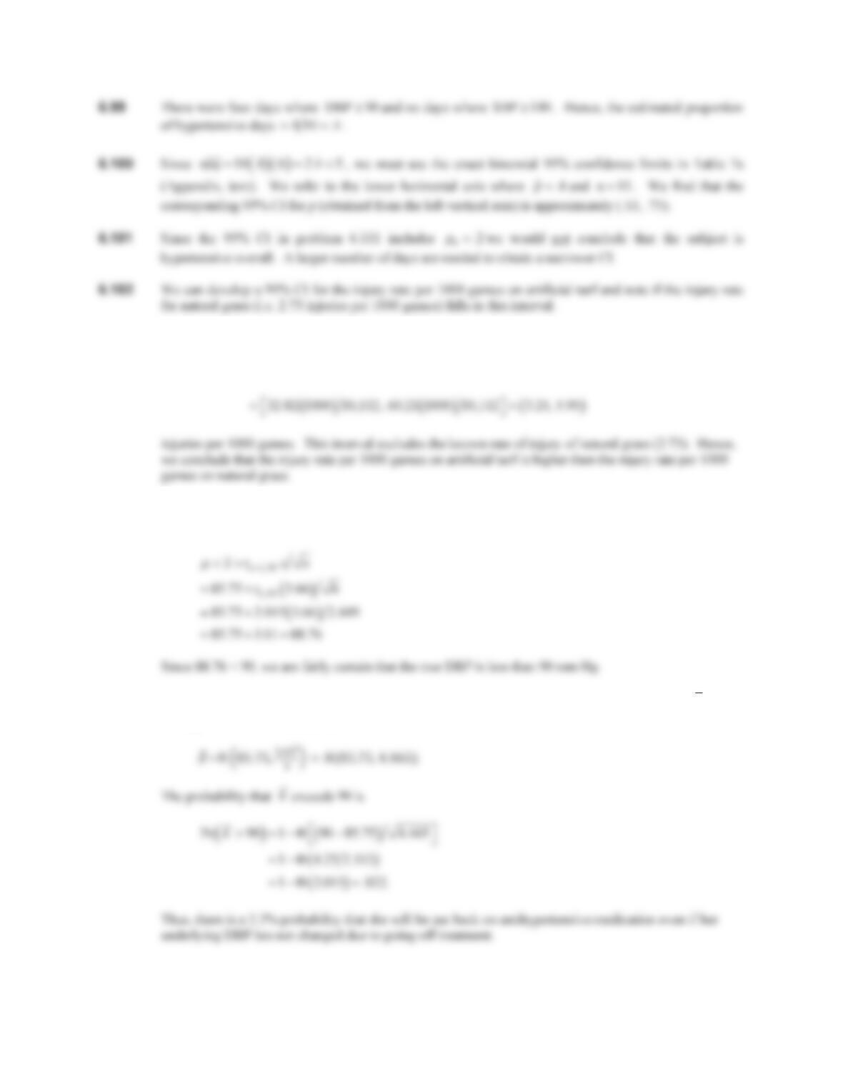
6.97 A 95% CI for mean SBP is given by
116 CHAPTER 6/ESTIMATION
6.103 We refer to Table 8 (Appendix, text). If the observed number of injuries 45X , then a 95% CI for the
expected number of injuries = (32.82, 63.23). The corresponding 95% CI for the rate of injuries per 1000
games
6.104 We construct a one-sided 95% CI for
P
where
P
is the underlying mean DBP for this woman while on
treatment. The interval is of the form
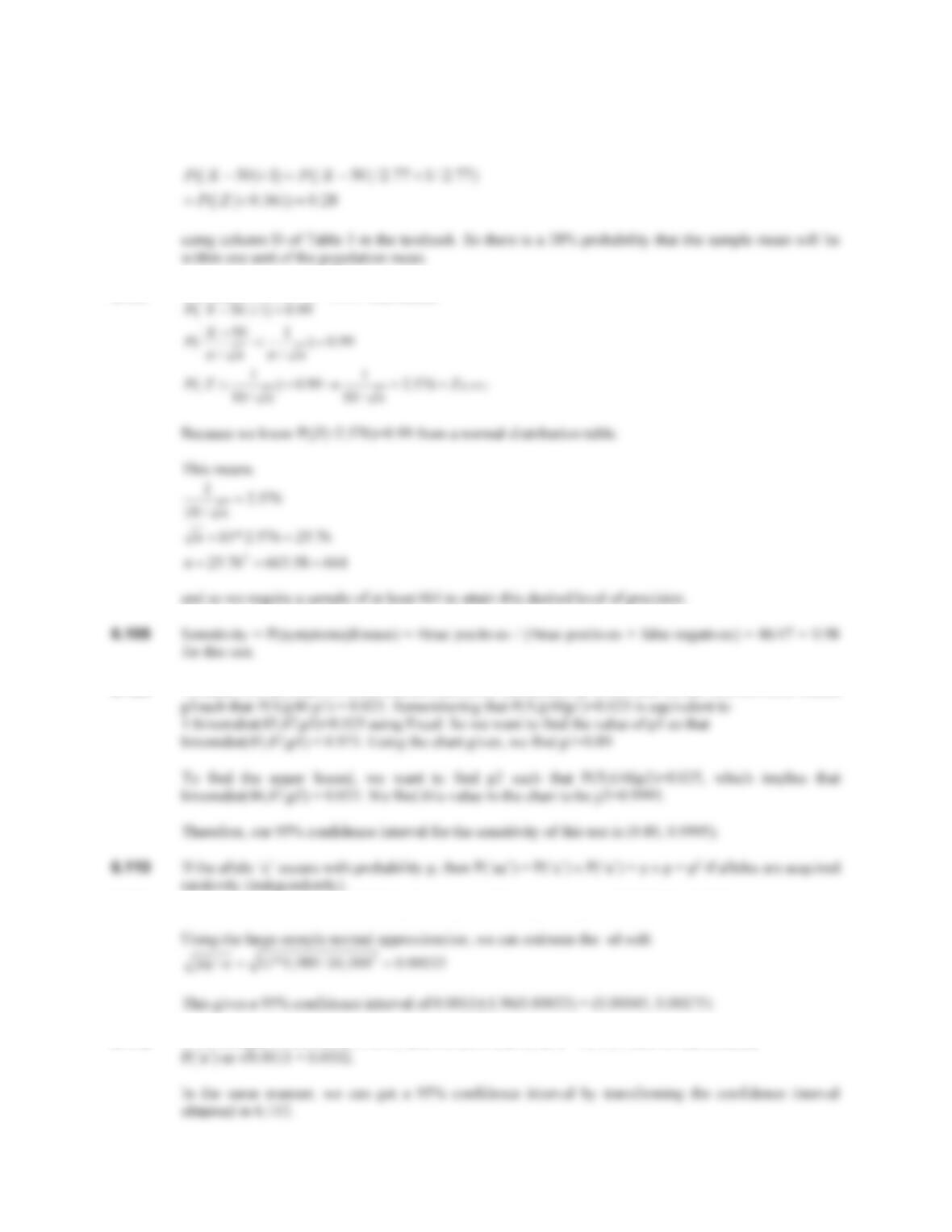
6.105 Let DBP
i
x for the ith week for this woman. We assume ̱ܺܰሺͺͷǤͷǡ͵Ǥଶሻ. Therefore, if
X
is the
average DBP over 3 weeks, then
X
CHAPTER 6/ESTIMATION 117
6.106 We know the sample mean of 13 observations also follows a normal distribution with mean = 50 and
standard deviation = 10/ξ13 = 2.77. Let X be a random variable with this distribution.
6.107 We want P(|X-50|<1) = 0.99. This means
6.109 To determine an exact 95% confidence interval for the sensitivity of the test, we can find the lower bound
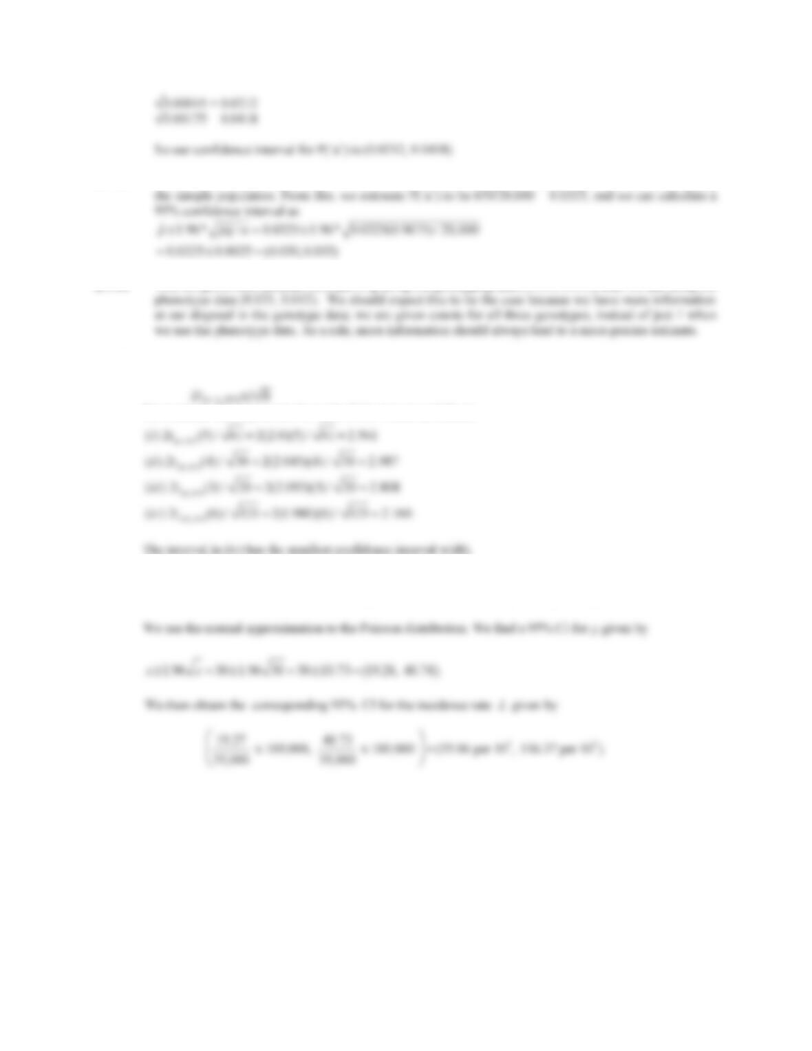
6.111 From this data, we estimate P(PKU phenotype) = P(‘aa’ genotype) = 11/10,000 = 0.0011
6.112 If we estimate P(‘aa’) to be 0.0011, and we know that P(‘aa’) = P(‘a’)2, then we can estimate
118 CHAPTER 6/ESTIMATION
6.113 Using this data, we find 630(1) + 10(2) = 650 ‘a’ alleles among 10,000(2) = 20,000 total alleles among
6.114 Yes, we get a more accurate estimate of p using the genotyping data (0.030, 0.035) than we did using the
6.115The95%confidenceintervalwidthisgivenby
Weevaluatethisexpressionforeachofthe4casesasfollows:
6.116 The estimated incidence rate = (30/35,000) x 100,000 = 85.71 cases per 105 person-years.