93
ESTIMATION
6.1 The treatments will be labeled as A and B and patients will be assigned to treatment A if the random digit
is from 0 to 4 inclusive and to treatment B if it is from 5 to 9 inclusive. Note that this method is one
among many possible randomization schemes that could be used. The treatment assignments given below
are obtained if one starts at the 28th row of Table 4 in the Appendix.
Patient
number
Random
digit
Treatment
assignment
1 6 B
2 9 B
3 6 B
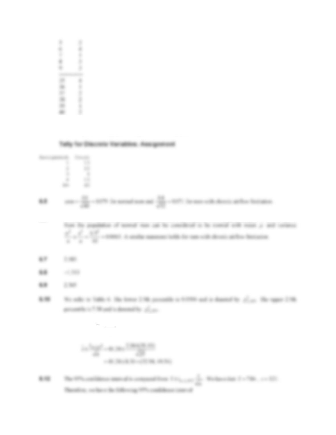
6.3 Here, we use the MINITAB command “Random Data”Æ “Discrete”, to generate 40 random numbers (1,
2, 3, 4), each drawn with probability 1/4 . Abbreviated output is shown below.
Pt. Assignment
1 4
94 CHAPTER 6/ESTIMATION
6.4` We expect to find 10 patients assigned to each treatment. For this particular example, we find the
following number of patients assigned to each treatment:
6.6 It means that the distribution of mean triceps skin-fold thickness from repeated samples of size 40 drawn
6.11 We have that
x 1031
25 41.24
years. Therefore, a 95% confidence interval for is given by
P
CHAPTER 6/ESTIMATION 95
6.13 A 90% confidence interval is given by
6.17 Since , we can use the normal theory method. Therefore, a 95% confidence
interval for the percentage of males discharged from Pennsylvania hospitals is given by
6.18 We have the following basic statistics:
P
6.19 A similar strategy is pursued for the common media data.
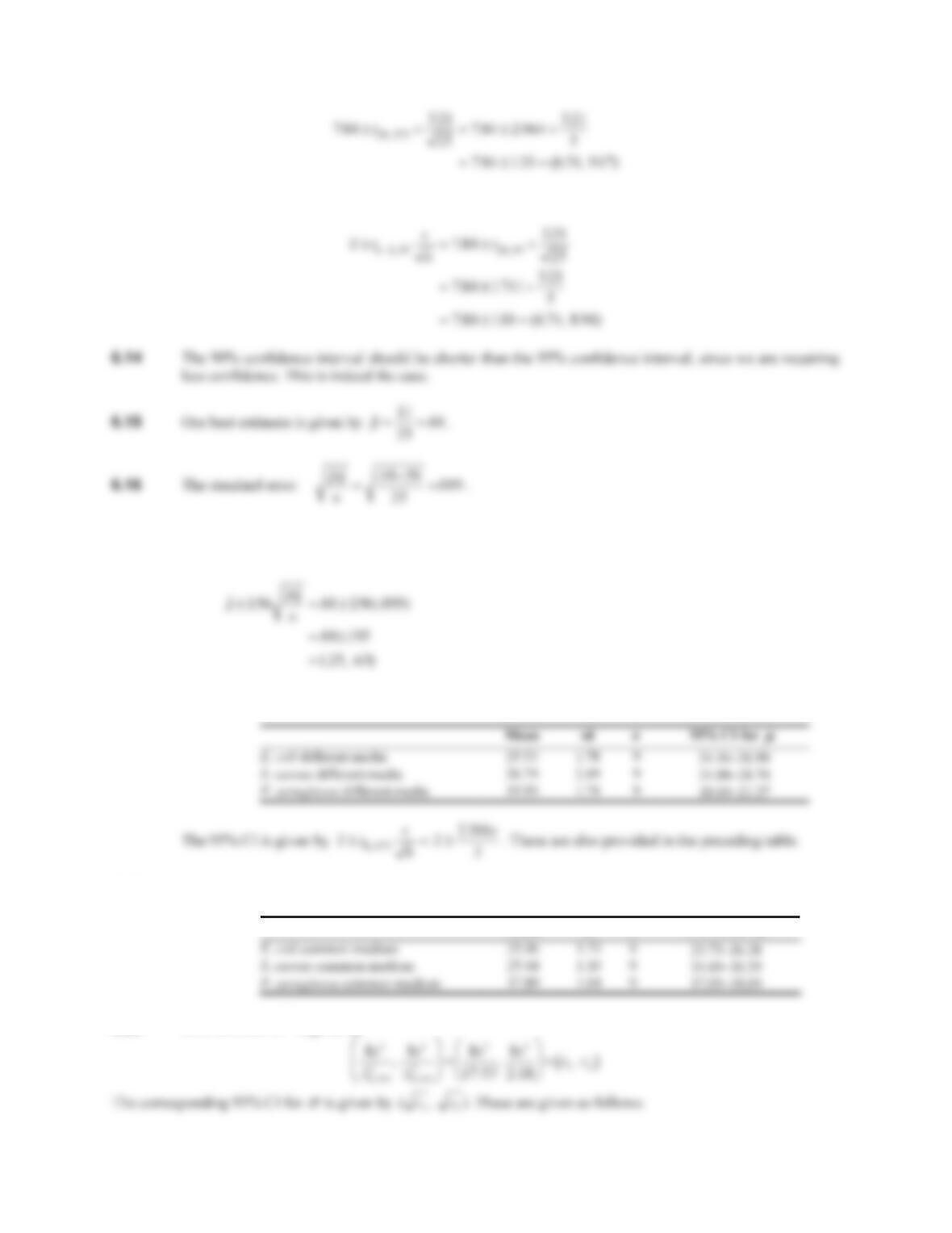
Mean sd n 95% CI for
6.20 A 95% CI for is given by
npq
.. . uu t25 44 56 616 5
P
V
2
96 CHAPTER 6/ESTIMATION
6.21 A similar approach is used for the common medium data. The results are:
Point estimate 95% CI for
6.23 The 95% CI is given by . For this purpose, we use the inverse CDF program of
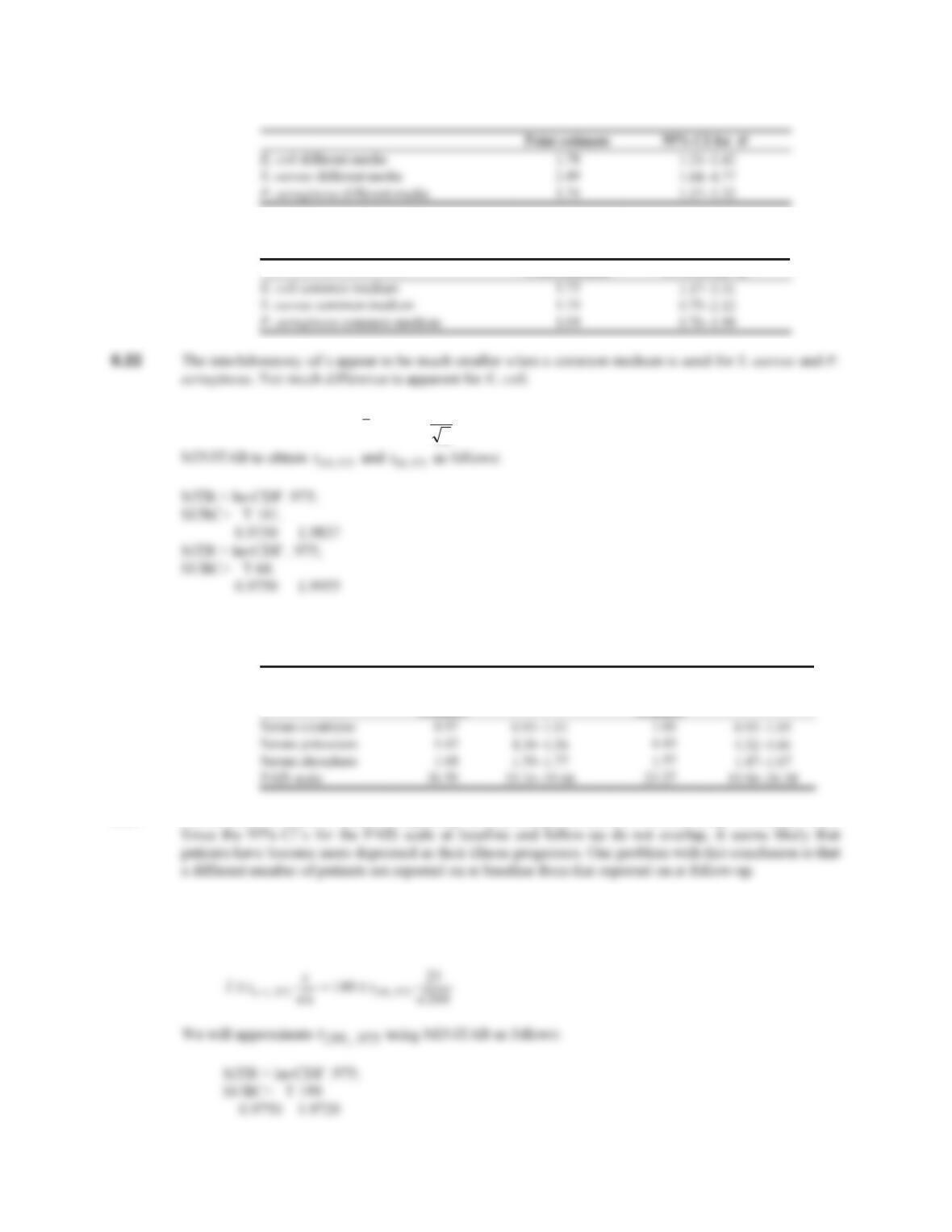
The point estimate and associated 95% CI are given as follows for each variable at baseline and follow-
up, respectively:
Baseline 18-month follow-up
Point
estimate
95% CI Point
estimate
95% CI
6.24 It is difficult to make a statement regarding the physiologic parameters without using two-sample tests.
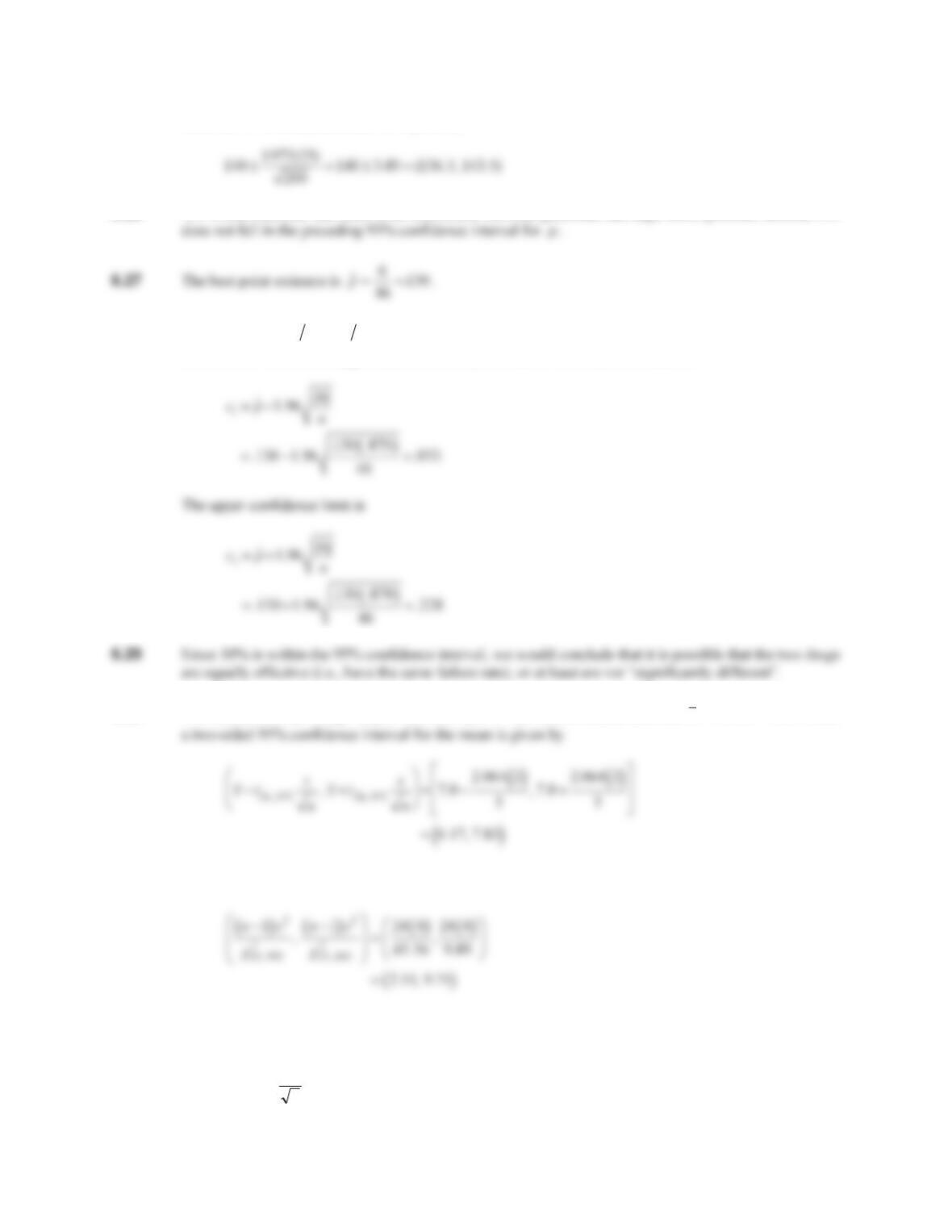
6.25 A 95% confidence interval for the true mean systolic blood pressure among people with glaucoma is
given by
V
xt s
n
n
r1 975,.
CHAPTER 6/ESTIMATION 97
Thus, the 95% confidence interval is given by
6.26 We would conclude that there is an association between glaucoma and high blood pressure because 130
P
6.28 Since
ˆˆ 46646 4046 5.2 5npq t
, we can use the normal approximation to the binomial
distribution. If a normal approximation is used, then the lower confidence limit is
6.30 We assume that ݔଵǡǥǡݔ
ଶହ̱ܰሺߤǡ ߪଶሻ, where , are unknown, and find that , . Thus,
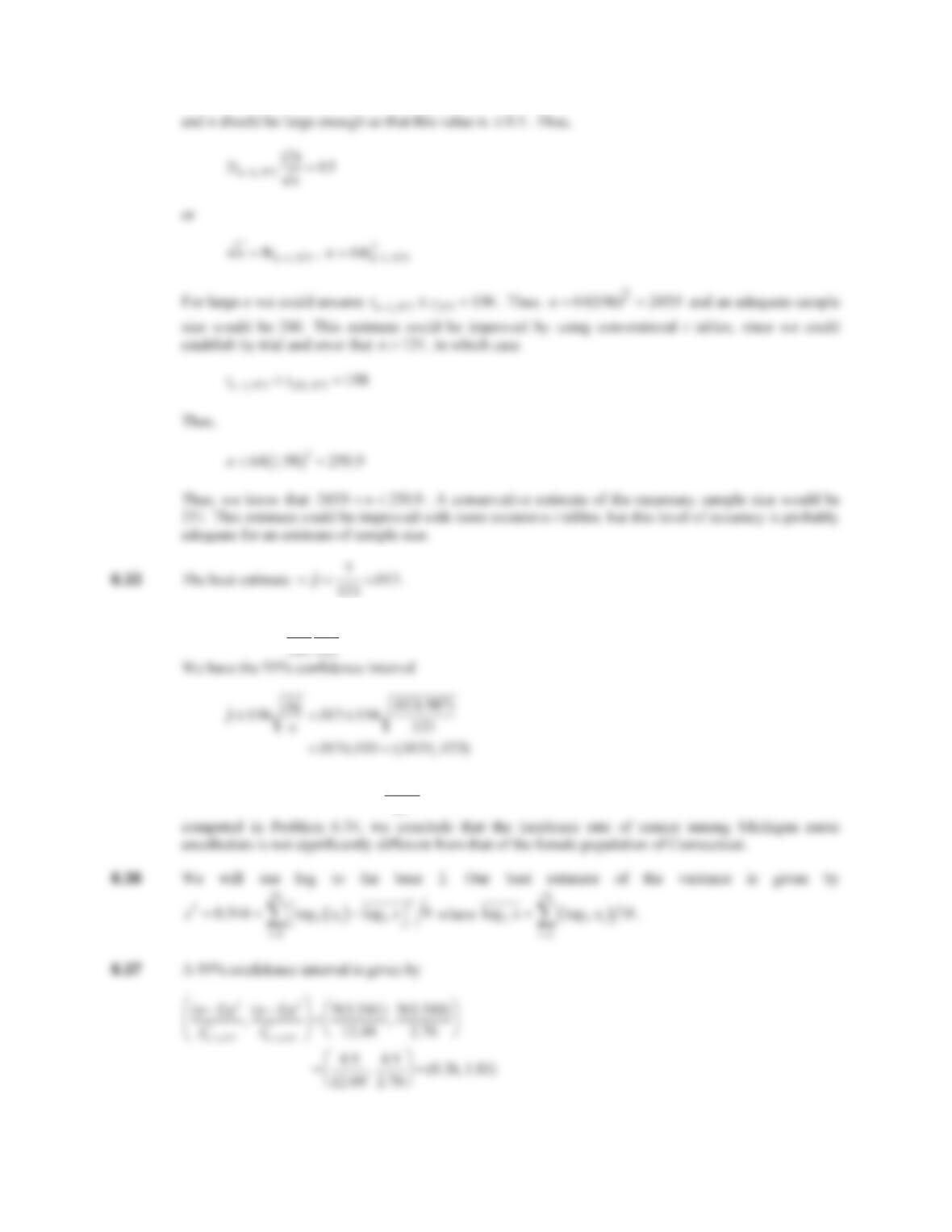
6.31 A two-sided 99% confidence interval for the unknown variance is given by
6.32 The length of the 95% confidence interval in Problem 6.41 is given by
P
V
2
x
70.
s
240 .
V
2
21 975
ts
n
n,.
98 CHAPTER 6/ESTIMATION
6.34 Since
nˆ
pˆ
q 525 7
518
, we can use the normal approximation method.
6.35 The expected incidence rate . Since this rate falls within the 95% confidence interval
402 8
10 0040
5
..
CHAPTER 6/ESTIMATION 99
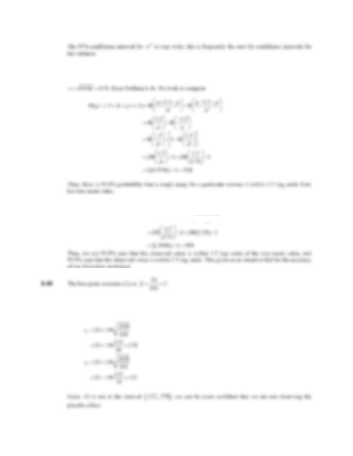
6.38 Suppose X is the observed value of an assay in the log scale, and is the “true” mean value.
We will assume that
X~N
P
,
V
2
, where variance of the assay. We approximate by
6.39 We want to compute
Pr(
P
2.5 X
P
2.5) 2)
P
2.5
P
V
§
©
¨
·
¹
¸1
of our laboratory technique.
6.41 We can compute the 95% confidence interval for p based on the normal approximation to the binomial
ˆˆ 16 5npq tand note if .10 falls in this interval. We have
P
V
2
V
100 CHAPTER 6/ESTIMATION
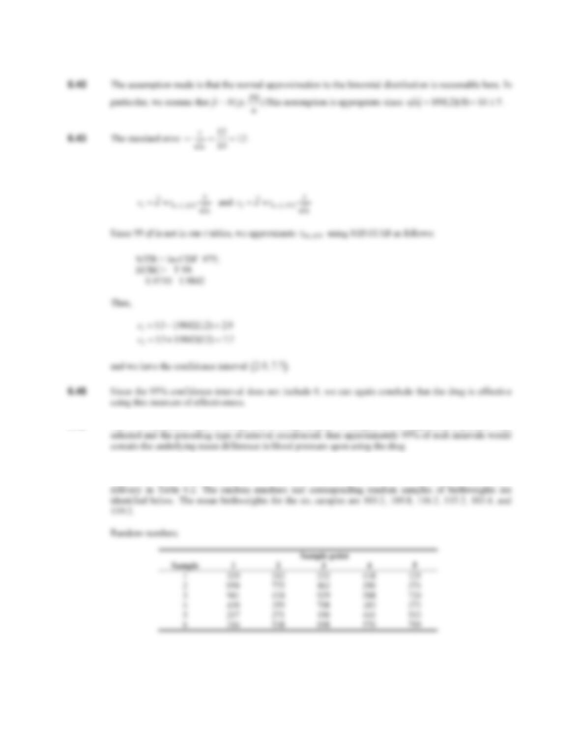
6.44 We can form a 95% confidence interval of the form
c
1
,c
2
based on the t distribution where
6.46 The 95% confidence interval means that if a large number of samples of 100 hypertensive patients were
6.47 The random samples can be selected in many different ways. The random numbers in Table 4 in the
Appendix will be used, starting in row 1, where each unique set of three digits identifies a unique
CHAPTER 6/ESTIMATION 101
Random samples of birthweights (oz)
Sample point
Sample 1 2 3 4 5 Mean
1 88 132 86 97 113 103.2
2 118 81 128 114 108 109.8
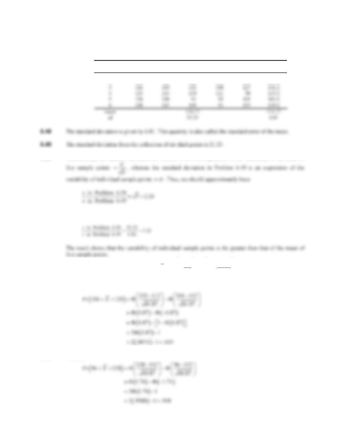
6.50 Theoretically, the standard deviation in Problem 6.48 is an expression of the variability of the mean of
6.51 Indeed,
6.52 If the central-limit theorem holds, then
XaN
P
,
V
2
n
§
©
¨
¨
·
¹
¸
¸ N112, 20.6
2
5
§
©
¨
¨
·
¹
¸
¸ N112, 84.87
. Therefore, it
follows that
6.53 We have
102 CHAPTER 6/ESTIMATION
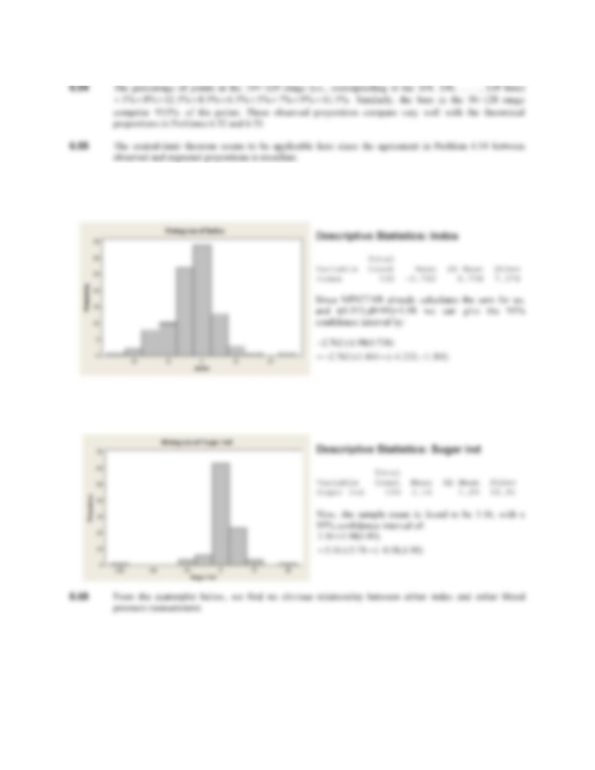
6.56 First, we calculate the variable “Index” as described in the question using trials 1-4. When we plot the
distribution, it appears to closely resemble a normal distribution. A histogram of the distribution is shown
below, along with descriptive statistics.
6.57 Here, we calculate “Sugar Index” = “msb3sug”-“msb2sug”. It is much less clear that these values can be
thought of as being normally distributed, primarily because of some extreme outliers. Histogram and
95% confidence interval for the mean are given below.
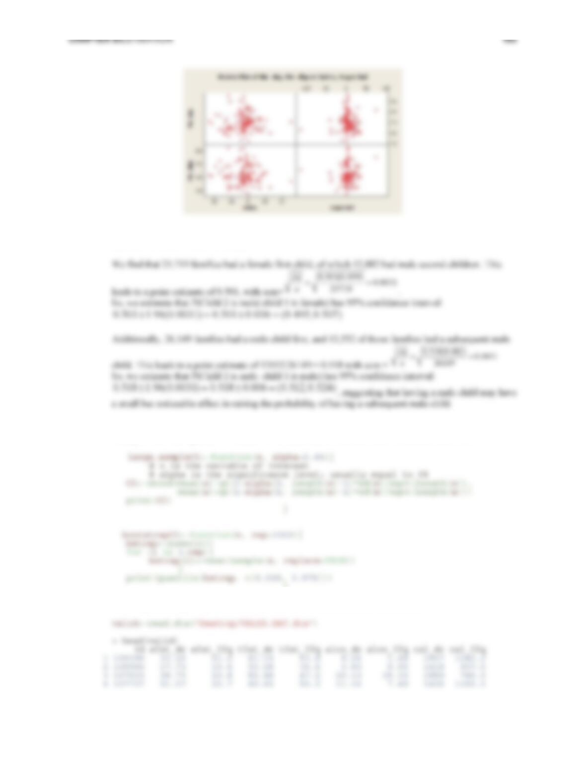
6.59 One way of addressing this problem is to estimate and compare P(Child 2 is male| Child 1 is female) with
P(Child 2 is male| Child 1 is male).
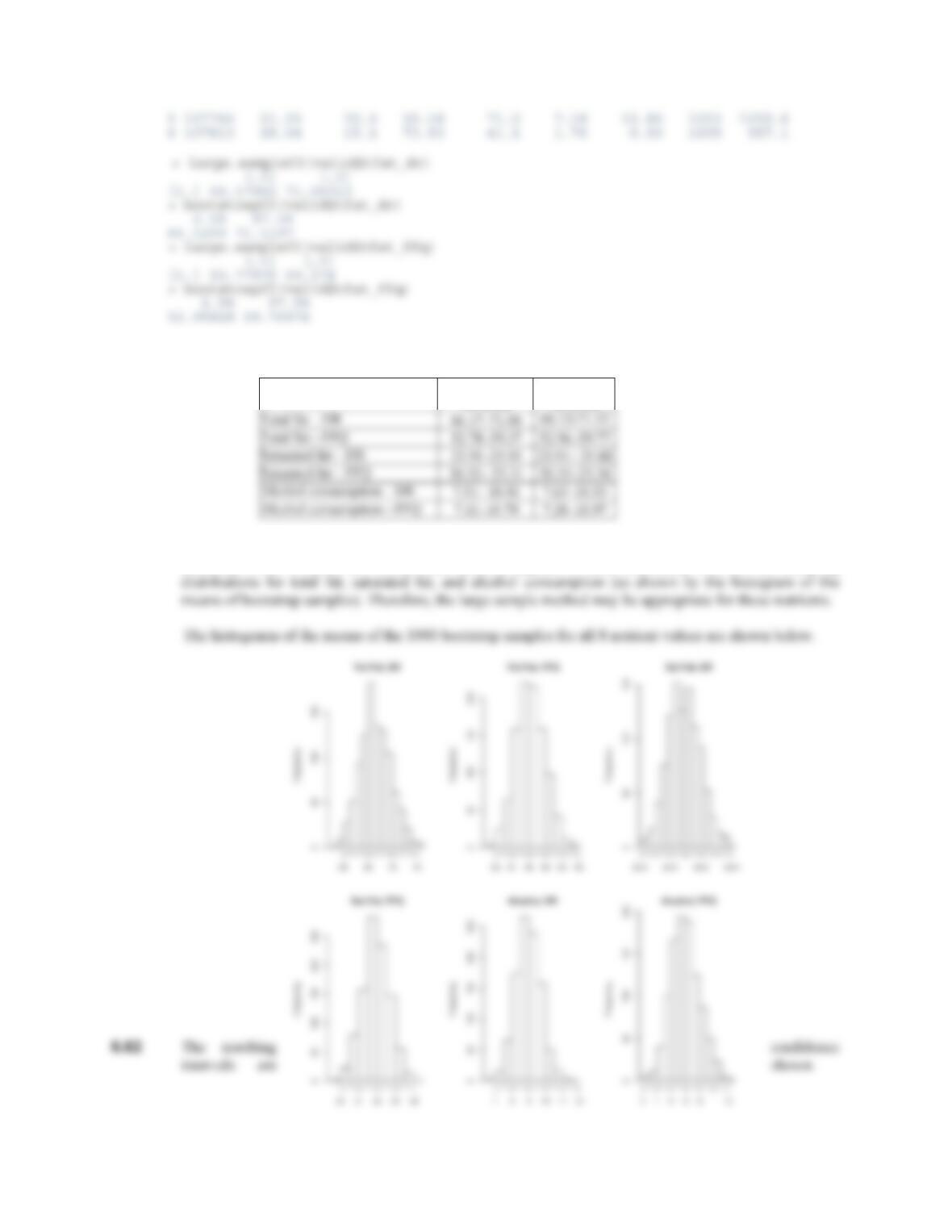
6.60 This problem can be addressed most efficiently by using a program like R, but can also be solved using a
variety of software options. We define two R functions to calculate these confidence intervals:
}
For example, the large sample and bootstrap confidence interval for the mean total fat are:
104 CHAPTER 6/ESTIMATION
We have the following results:
Large sample
95% CI
Bootstrap
95% CI
6.61 For each nutrient, the large sample confidence intervals and the bootstrap confidence intervals are
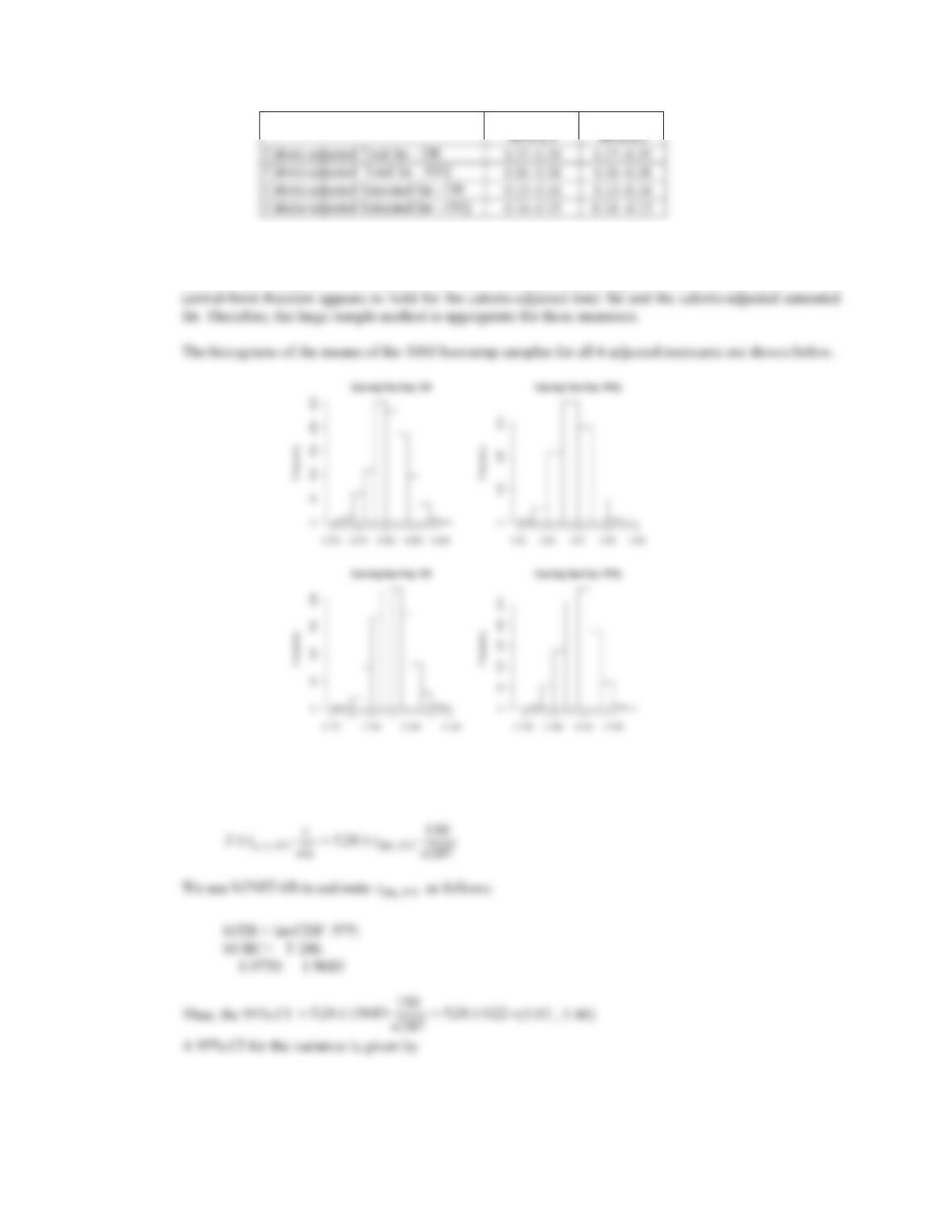
relatively close. Overall, the central-limit theorem appears to hold reasonably well for the sampling
CHAPTER 6/ESTIMATION 105
Large sample
Bootstrap
6.63
The large sample and bootstrap confidence intervals are equal for each adjusted measure of nutrients. In
addition, the histogram of the means of the 1000 bootstrap samples appear to be fairly symmetric, i.e. the
6.64 The mean latency time years with years, and sample size = 287. Thus, a 95% CI for the
mean is given by
524.
s
d 190.