CHAPTER 6
SOLUTIONS TO EXERCISES—SET B
EXERCISE 6-1B
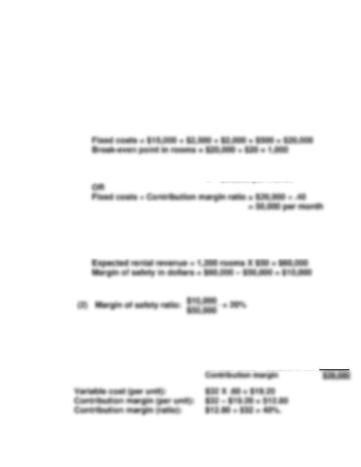
(a) (1) Contribution margin per room = $50 – ($5 + $25)
Contribution margin per room = $20
Contribution margin ratio = $20 ÷ $50 = 40%
(2) Break-even point in dollars = 1,000 rooms X $50 per room
= $50,000 per month
(b) (1) Margin of safety in dollars:
Planned activity = 40 rooms per day X 30 days
= 1,200 rooms per month
EXERCISE 6-2B
(a) Contribution margin (in dollars): Sales = (3,100 X $32) = $99,200
Variable costs = $99,200 X .60 = 59,520
EXERCISE 6-2B (Continued)
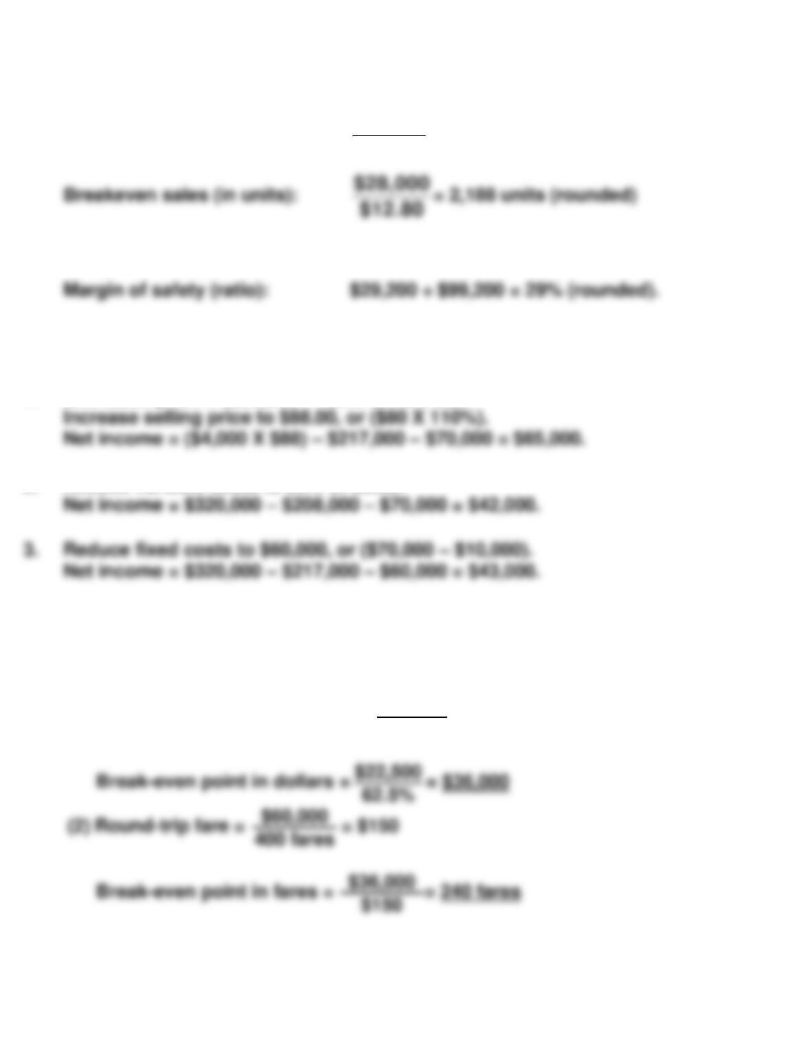
(b) Breakeven sales (in dollars):
$28,000
40%
= $70,000
(c) Margin of safety (in dollars): $99,200 – $70,000 = $29,200.
EXERCISE 6-3B
1. Unit sales price = $320,000 ÷ 4,000 units = $80
2. Reduce variable costs to 65% of sales.
Alternative 1, increasing selling price, will produce the highest net income.
EXERCISE 6-4B
(a)
(1) Contribution margin ratio is:
$37,500
= 62.5%
$60,000
EXERCISE 6-4B (Continued)
(b) At the break-even point fixed costs and contribution margin are equal.
Therefore, the contribution margin at the break-even point would be
$22,500.
(c)
Fare revenue ($135* X 480**) ………………
$64,800
Variable costs ($22,500 X 1.20) …………..
27,000
EXERCISE 6-5B
DARRON COMPANY
CVP Income Statement (Current)
For the Year Ended December 31, 2017
Total
Per Unit
Sales (50,000 X $25) …………………………………
$1,250,000
$25
Contribution margin ………………………….
Fixed costs ……………………………………….
Net income ……………………………………….
EXERCISE 6-5B (Continued)
DARRON COMPANY
CVP Income Statement (with Changes)
For the Year Ended December 31, 2017
Total
Per Unit
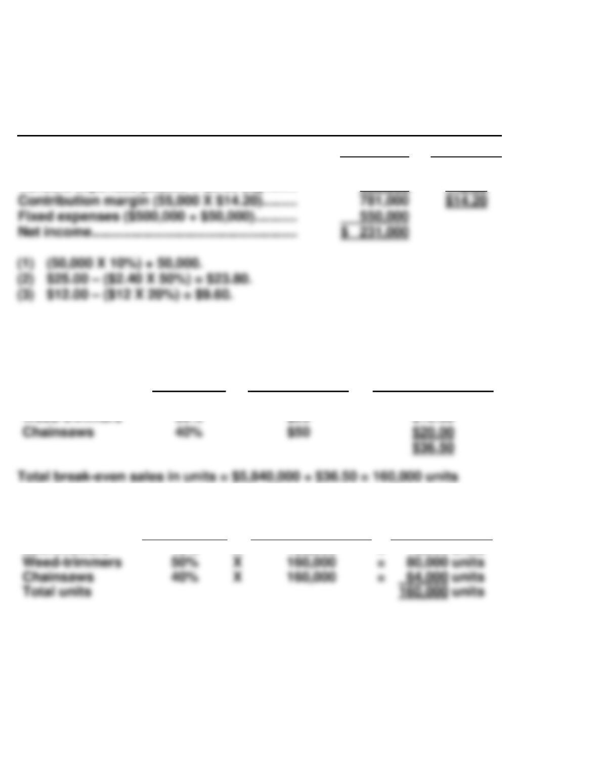
Sales [55,000 units (1) X $23.80 (2)] ………….
Variable expenses [55,000 X $9.60 (3)] ……..
$1,309,000
528,000
$23.80
9.60
EXERCISE 6-6B
Sales Mix
Percentage
Contribution
Margin Per Unit
Weighted-Average
Contribution Margin
Lawnmowers
10%
$40
$4.00
Sales Mix
Percentage
Total
Break-even Sales
in Units
Sales Units
Needed
Per Product
Lawnmowers
10%
X
160,000
=
16,000 units
EXERCISE 6-7B
(a)
Sales Mix
Percentage
Contribution
Margin Ratio
Weighted-Average
Contribution
Margin Ratio
Oil changes
70%
20%
.14
Sales Mix
Percentage
Total
Break-even Sales
in Dollars
Sales Dollars
Needed
Per Product
Total sales
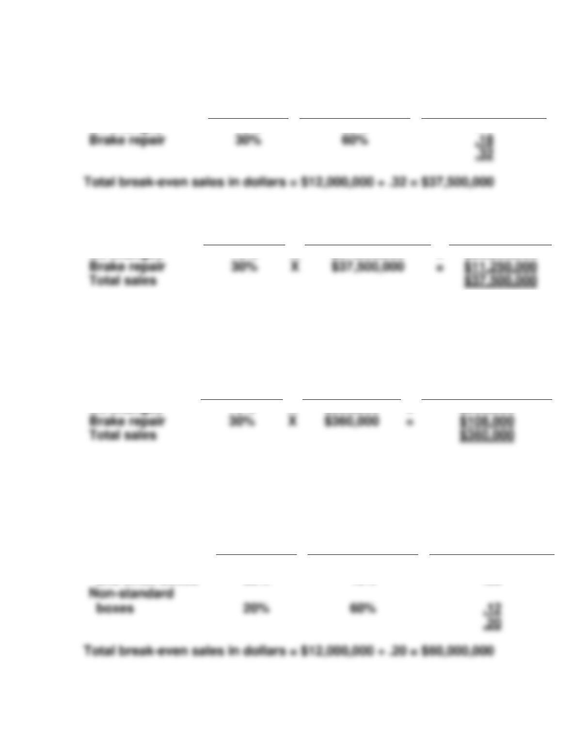
Oil changes
70%
X
$37,500,000
=
$26,250,000
(b)
Sales to achieve target net income = ($40,000 + $75,200) ÷ .32 = $360,000
Sales Mix
Percentage
Total
Sales Needed
Sales Dollars
Needed Per Product
Per Store
Total sales
Oil changes
70%
X
$360,000
=
$252,000
EXERCISE 6-8B
(a)
Sales Mix
Percentage
Contribution
Margin Ratio
Weighted-Average
Contribution
Margin Ratio
Mail pouches
and small boxes
80%
10%
.08
EXERCISE 6-8B (Continued)
Sales Mix
Percentage
Total Break-
even Sales
in Dollars
Sales Dollars
Needed
Per Product
Mail pouches
and small boxes
80%
X
$60,000,000
=
$48,000,000
(b)
Sales Mix
Percentage
Contribution
Margin Ratio
Weighted-Average
Contribution
Margin Ratio
Non-standard
Mail pouches
Sales Mix
Percentage
Total Break-
even Sales
in Dollars
Sales Dollars
Per Product
Total sales
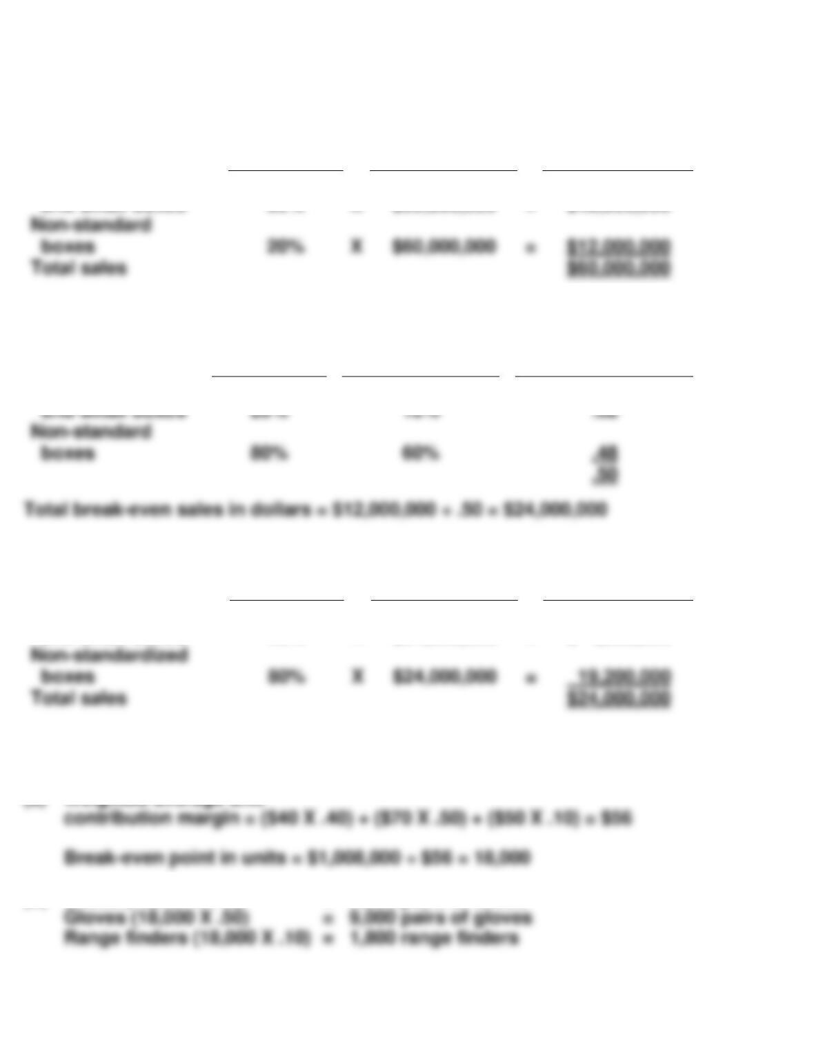
Mail pouches
and small boxes
20%
X
$24,000,000
=
$ 4,800,000
EXERCISE 6-9B
(a) Weighted-average unit
(b) Shoes (18,000 X .40) = 7,200 pairs of shoes
Non-standard
Total sales
$60,000,000
EXERCISE 6-9B (Continued)
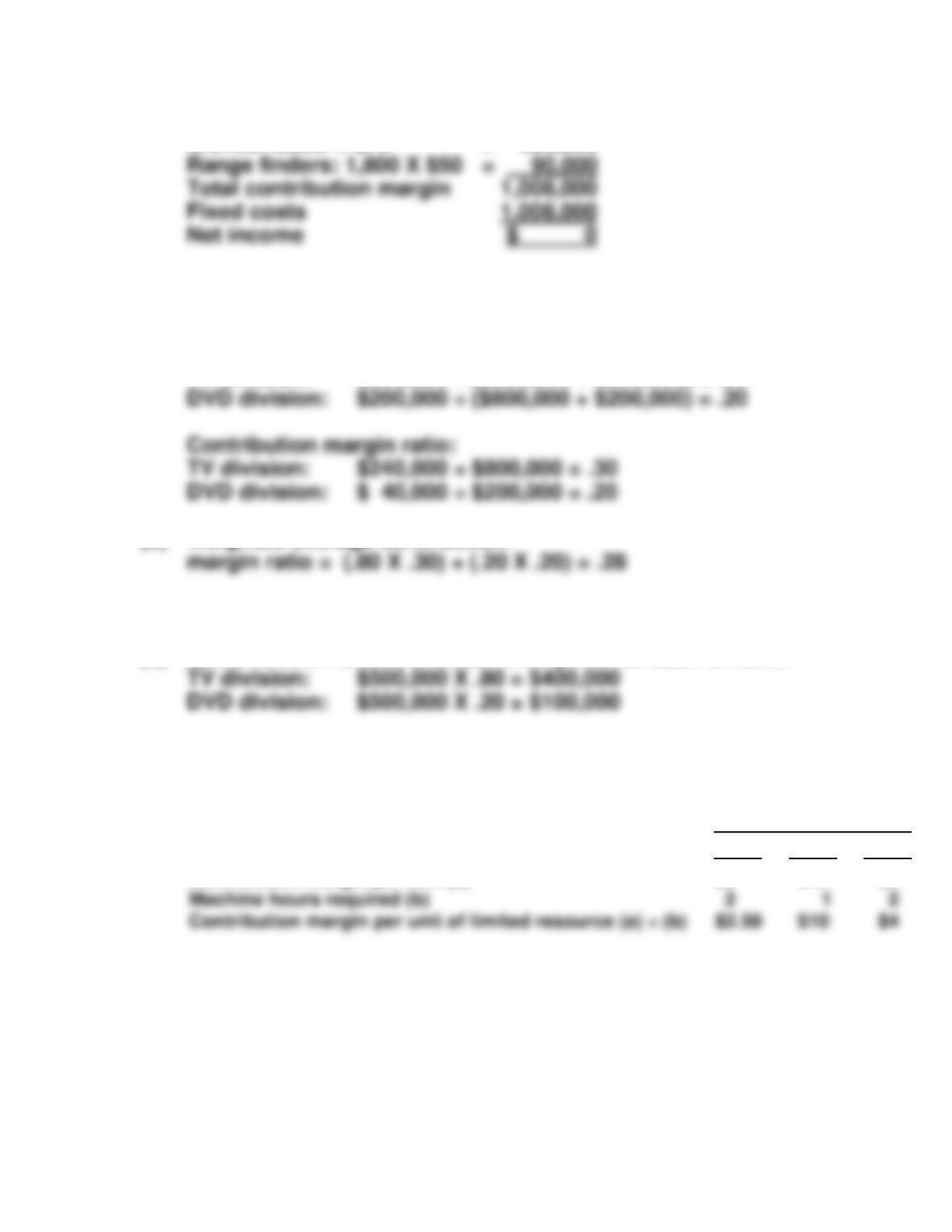
(c) Shoes: 7,200 X $40 = $288,000
Gloves: 9,000 X $70 = 630,000
EXERCISE 6-10B
(a) Sales mix percentage
TV division: $800,000 ÷ ($800,000 + $200,000) = .80
(b) Weighted-average contribution
(c) Break-even point in dollars = $140,000 ÷ .28 = $500,000
(d) Sales dollars needed at break-even point for each division
EXERCISE 6-11B
(a)
Product
A
B
C
Contribution margin per unit of limited resource (a) ÷ (b)
$2.50
Contribution margin per unit (a)
$5
$10
$8
(b) Product B should be manufactured because it results in the highest
contribution margin per machine hour.
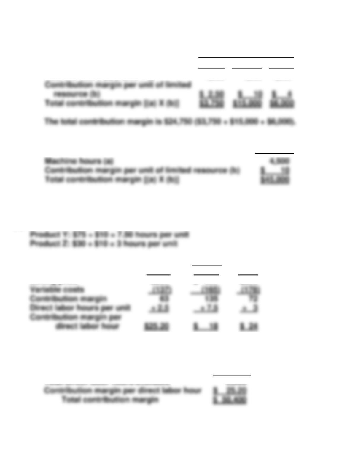
EXERCISE 6-11B (Continued)
(c)
(1)
Product
A
B
C
Machine hours (a) (4,500 ÷ 3)
1,500
1,500
1,500
(2)
Product
B
Total contribution margin [(a) X (b)]
EXERCISE 6-12B
(a)
Product X: $25 ÷ $10 = 2.50 hours per unit
Product Y: $75 ÷ $10 = 7.50 hours per unit
Product Z: $30 ÷ $10 = 3 hours per unit
(b)
Product
X
Y
Z
Selling price
$200
$ 300
$250
Variable costs
Contribution margin
Direct labor hours per unit
÷ 7.5
Contribution margin per
direct labor hour
(c) Product X should be produced because it generates the highest contri–
bution margin per direct labor hour.
Product X
Total direct labor hours available
2,000
Contribution margin per direct labor hour
Total contribution margin
Total contribution margin [(a) X (b)]
$3,750
$15,000
$6,000
EXERCISE 6-13B
(a)
Product
Basic
Deluxe
Selling price per unit
$40
$52
(b) The Basic product should be manufactured because it results in the
higher contribution margin per machine hour.
(c)
(1)
Basic
Deluxe
Total
Machine hours allocated
500
500
1,000
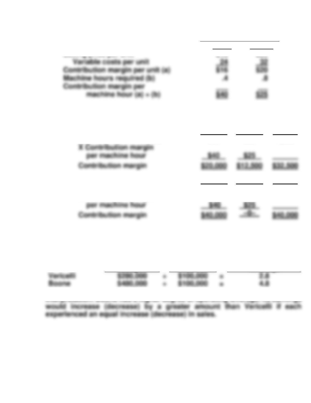
X Contribution margin
(2)
Basic
Deluxe
Total
Machine hours allocated
1,000
–0–
1,000
per machine hour
X Contribution margin
EXERCISE 6-14B
(a)
Contribution
Margin
÷
Net
Income
=
Degree of Operating
Leverage
Vericelli
Boone
÷
÷
=
=
Contribution margin per unit (a)
Machine hours required (b)
Contribution margin per
machine hour (a) ÷ (b)
EXERCISE 6-14B (Continued)
(b)
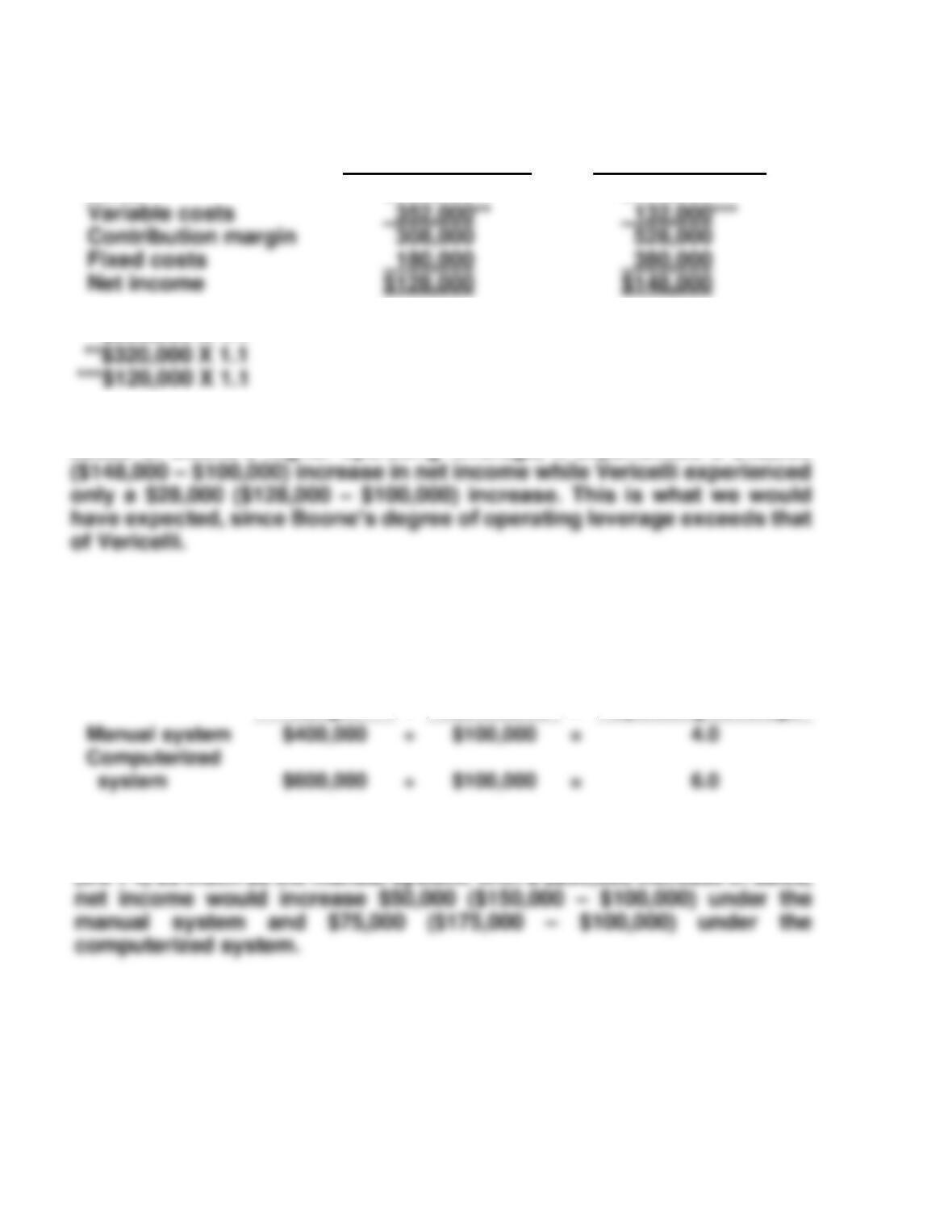
Vericelli Company
Boone Company
Sales
$660,000**
$660,000***
*$600,000 X 1.1
(c) Each company experienced a $60,000 increase in sales. However, be–
cause of Boone’s higher operating leverage, it experienced a $48,000
EXERCISE 6-15B
(a)
Contribution
Margin
÷
Net Income
=
Degree of
Operating Leverage
Computerized
÷
=
(b) The computerized system would produce profits that are 1.5 times
EXERCISE 6-15B (Continued)
Manual
System
Computerized
System
Sales
Variable costs
$1,800,000
1,350,000*
$1,800,000
1,125,000**
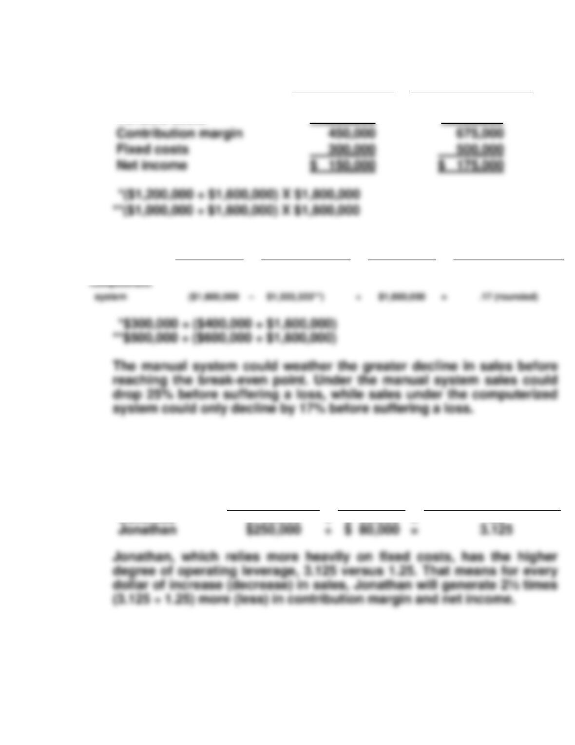
(c)
(Actual Sales
–
Break-even Sales)
÷
Actual Sales
=
Margin of Safety Ratio
–
÷
=
Manual system
($1,600,000
–
$1,200,000*)
÷
$1,600,000
=
.25
EXERCISE 6-16B
(a)
Contribution
Margin
÷
Net
Income
=
Degree of Operating
Leverage
Jonathan
÷
=
Delicious
$100,000
÷
$ 80,000
=
1.25
EXERCISE 6-16B (Continued)
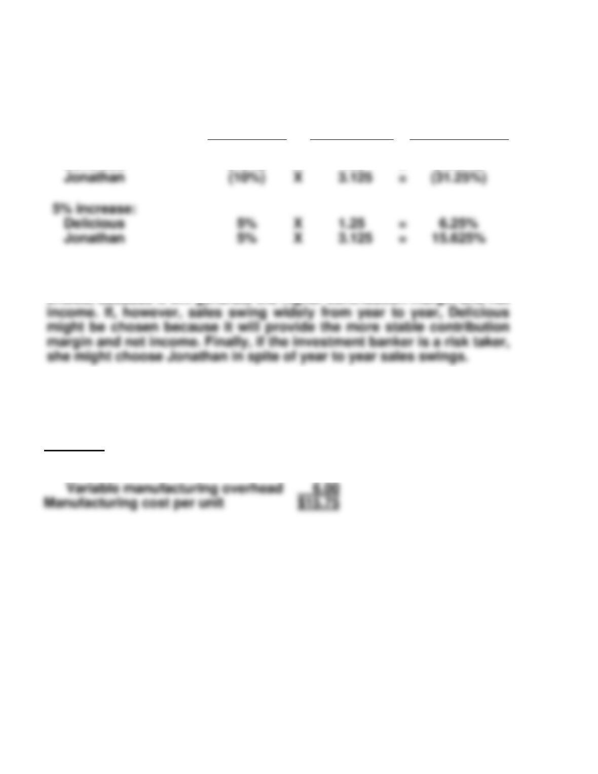
(b)
% Change
in Sales
X
Degree of
Operating
Leverage
=
% Change in
Net Income
10% decrease:
Delicious
(10%)
X
1.25
=
(12.5%)
(c) There are several possible answers that could be given. For example, if
the candied apple business is fairly stable, Jonathan might be the
choice, because it will generate the higher contribution margin and net
*EXERCISE 6-17B
(a)
Unit Cost
Direct materials
$ 7.50
Direct labor
2.25
6.00
Manufacturing cost per unit
$15.75
Jonathan
X
=
*EXERCISE 6-17B (Continued)
(b)
KARE COMPANY
Income Statement
For the Year Ended December 31, 2017
Variable Costing
Sales (80,000 lures X $28) …………………….
$2,240,000
Variable cost of goods sold
(80,000 lures X $15.75) ……………………….
$1,260,000
(c)
Unit Cost
Direct materials ……………………………………………..
$ 7.50
Direct labor …………………………..………………………
2.25
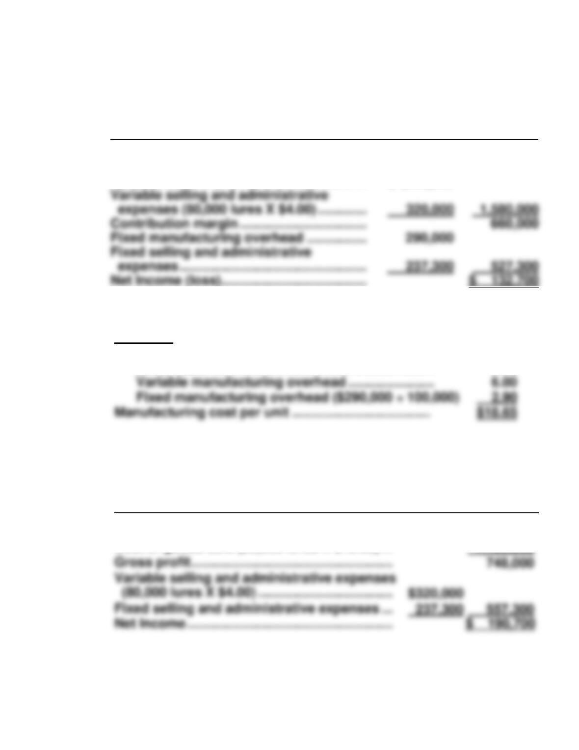
Variable manufacturing overhead …………………..
Fixed manufacturing overhead ($290,000 ÷ 100,000)
2.90
Manufacturing cost per unit ……………………………….
(d)
KARE COMPANY
Income Statement
For the Year Ended December 31, 2017
Absorption Costing
Sales (80,000 lures X $28) ………………………….
$2,240,000
Cost of goods sold (80,000 lures X $18.65) …
1,492,000
Gross profit ………………………………………………
Fixed selling and administrative expenses …
557,300
Net Income ……………………………………………….
Variable selling and administrative
expenses (80,000 lures X $4.00) ………….
320,000
Contribution margin …………………………….
Fixed manufacturing overhead …………….
Fixed selling and administrative
expenses …………………………..………………
Net Income (loss)…………………………………
*EXERCISE 6-18B
(a) Direct materials used $ 85,000
Direct labor incurred 30,000
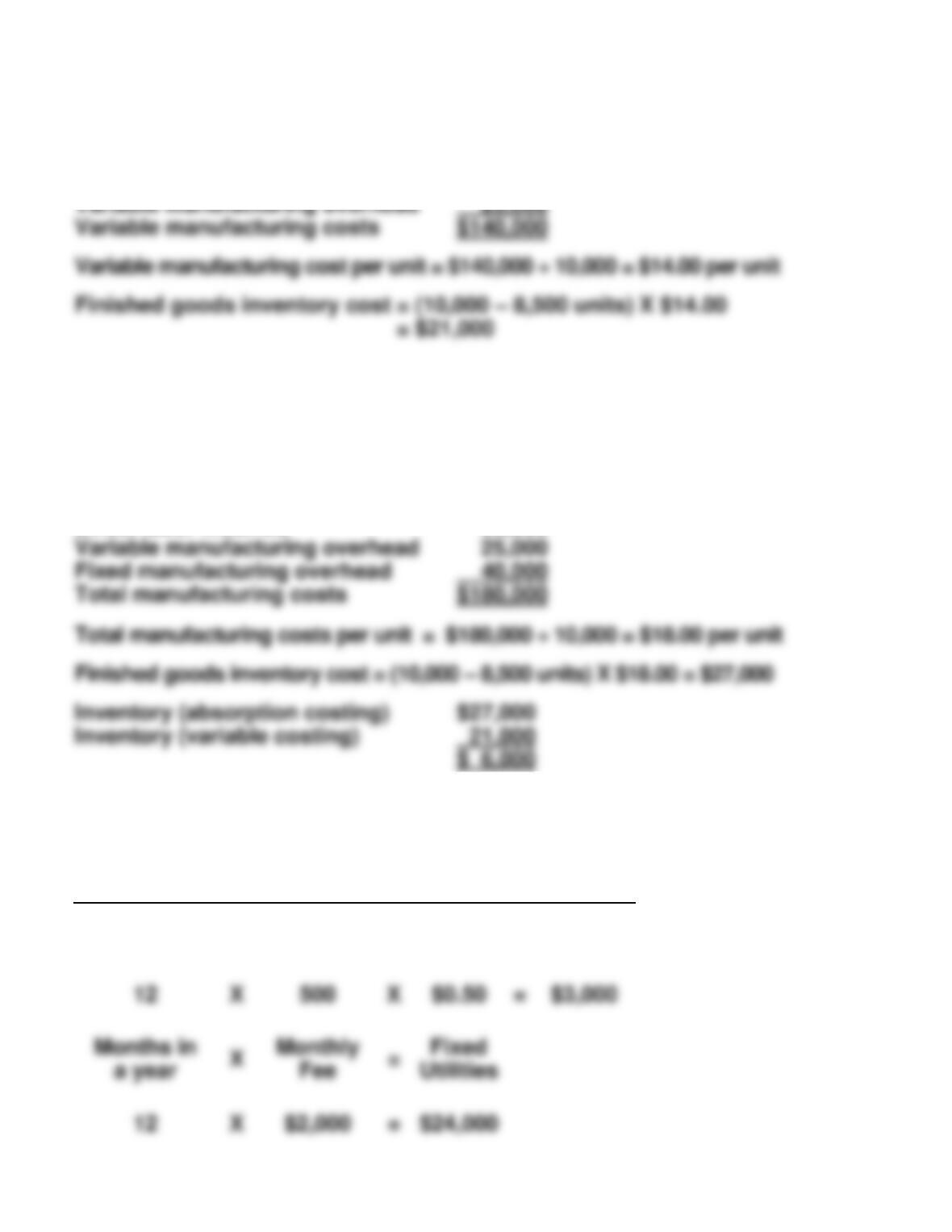
(b) Absorption costing would show a higher net income because a portion
of the fixed costs are deferred to future periods. The following
computation indicates that finished goods inventory will be $6,000
higher under absorption costing which will cause its net income to be
$6,000 higher.
Direct materials used $ 85,000
Direct labor incurred 30,000
*EXERCISE 6-19B
(a)
Utility Expense
Months in
a year
X
Kilowatt
hours
X
Hourly
Charge
=
Variable
Utilities
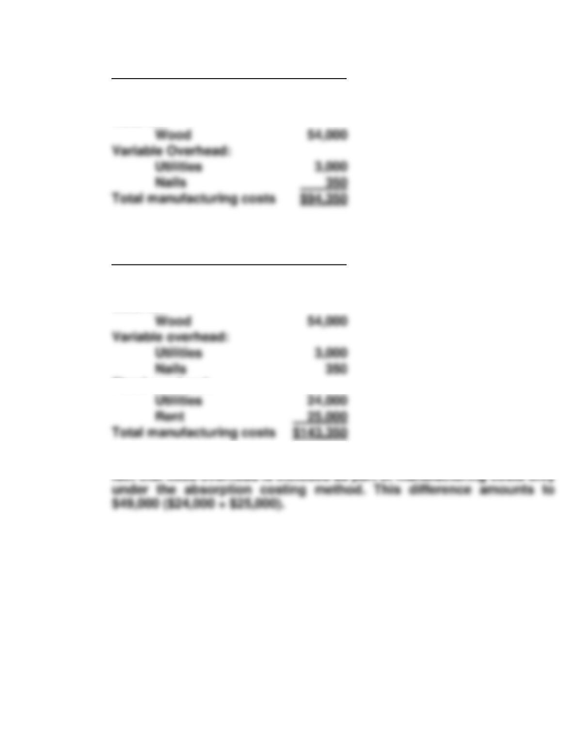
*EXERCISE 6-19B (Continued)
Variable Costing
Labor:
Crate builders
$37,000
Material:
(b)
Absorption Costing
Labor:
Crate builders
$ 37,000
Material:
Variable overhead:
Utilities
Fixed overhead:
Utilities
Total manufacturing costs
(c) The entire difference in costs between the two methods is due to the
Wood
Variable Overhead:
Nails
Total manufacturing costs
$94,350
SOLUTIONS TO PROBLEMS—SET C
PROBLEM 6-1C
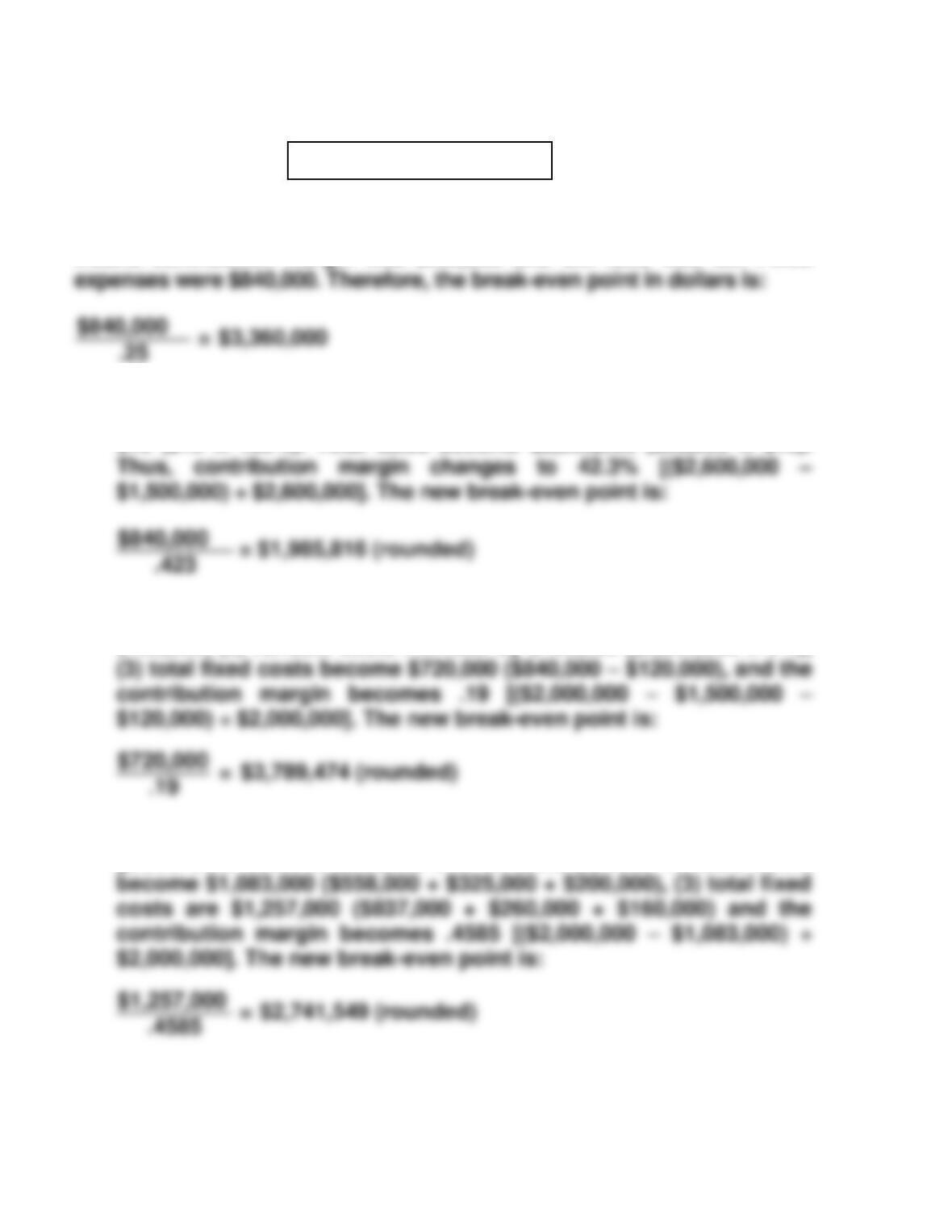
(a) Sales were $2,000,000 and variable expenses were $1,500,000, which
means contribution margin was $500,000 and CM ratio was .25. Fixed
(b) (1) The effect of this alternative is to increase the selling price per unit to
$13 ($10 X 130%). Total sales become $2,600,000 (200,000 X $13).
(2) The effects of this alternative are: (1) fixed costs decrease by
$120,000, (2) variable costs increase by $120,000 ($2,000,000 X 6%),
(3) The effects of this alternative are: (1) variable and fixed cost of
goods sold become $558,000 and 837,000, (2) total variable costs
Alternative 1 is the recommended course of action using break-even
analysis because it has the lowest break-even point.
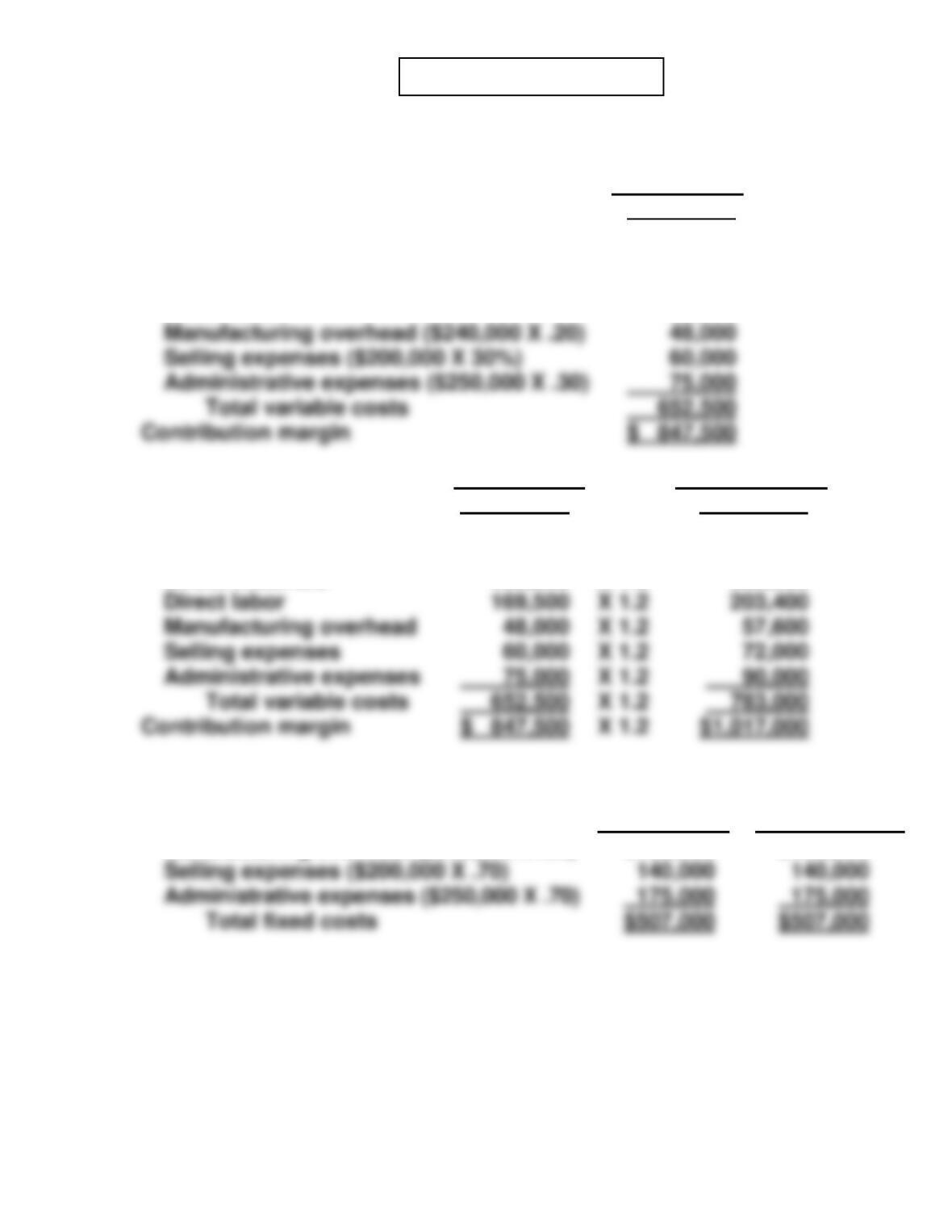
PROBLEM 6-2C
(a)
(1)
Current Year
Sales
Variable costs
Direct materials
Direct labor
$1,500,000
300,000
169,500
Current Year
Projected Year
Contribution margin
Sales
Variable costs
Direct materials
$1,500,000
300,000
X 1.2
X 1.2
$1,800,000
360,000
(2)
Fixed Costs
Current Year
Projected year
Total fixed costs
Manufacturing overhead ($240,000 X .80)
$192,000
$192,000
Selling expenses ($200,000 X 30%)
Contribution margin
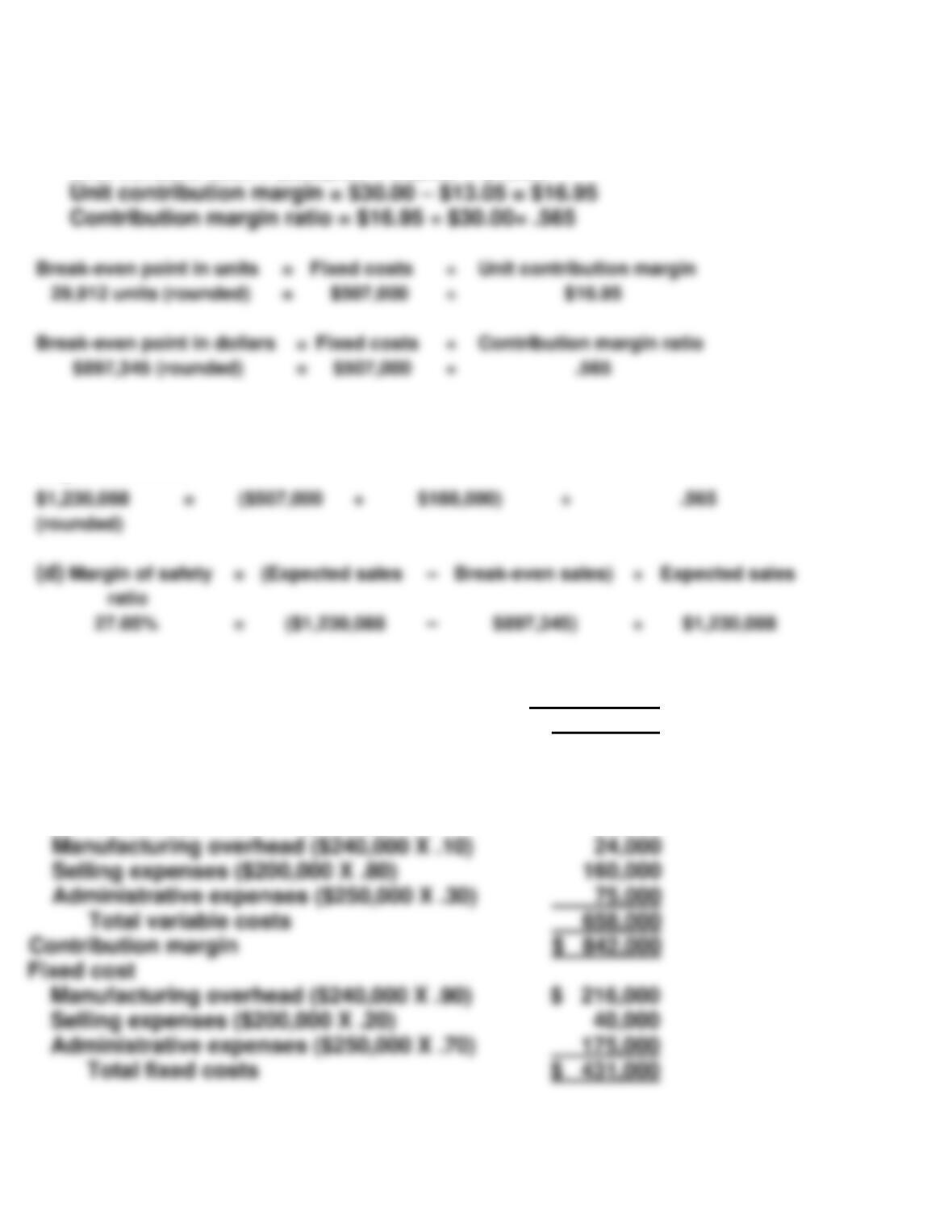
PROBLEM 6-2C (Continued)
(b) Unit selling price = $1,500,000 ÷ 50,000 = $30.00
Unit variable cost = $652,500 ÷ 50,000 = $13.05
(c) Sales dollars
required for
=
(Fixed costs
+
Target net income)
÷
Contribution margin ratio
target net income
(rounded)
ratio
=
÷
(e)
(1)
Current Year
Contribution margin
Total fixed costs
Sales
Variable costs
Direct materials
Direct labor ($169,500 – $70,500)
$1,500,000
300,000
99,000
Break-even point in units
=
Fixed costs
÷
Unit contribution margin
=
÷
Break-even point in dollars
=
Fixed costs
÷
Contribution margin ratio
=
÷
PROBLEM 6-2C (Continued)
(3) Break-even point in dollars = $431,000 ÷ .561 = $768,271 (rounded)
The break-even point in dollars declined from $897,345 to $768,271. This
means that overall the company’s risk has declined because it doesn’t
have to generate so much in sales. The two changes actually had
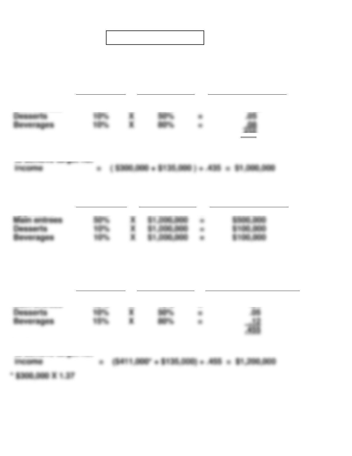
PROBLEM 6-3C
(a)
Sales Mix
Percentage
X
Contribution
Margin Ratio
=
Weighted-Average
Contribution
Margin Ratio
Appetizers
Main entrees
30%
50%
X
X
60%
25%
=
=
.18
.125
.435
Total sales required
Sales Mix
Percentage
X
Total Sales
=
Sales from
Each Product
Main entrees
Desserts
Beverages
X
X
X
=
=
=
Appetizers
30%
X
$1,000,000
=
$300,000
(b)
Sales Mix
Percentage
X
Contribution
Margin Ratio
=
Weighted-Average
Contribution
Margin Ratio
Desserts
Beverages
X
X
=
=
Appetizers
Main entrees
35%
40%
X
X
70%
10%
=
=
.245
.04
Total sales required
to achieve target net
Desserts
Beverages
X
X
=
=
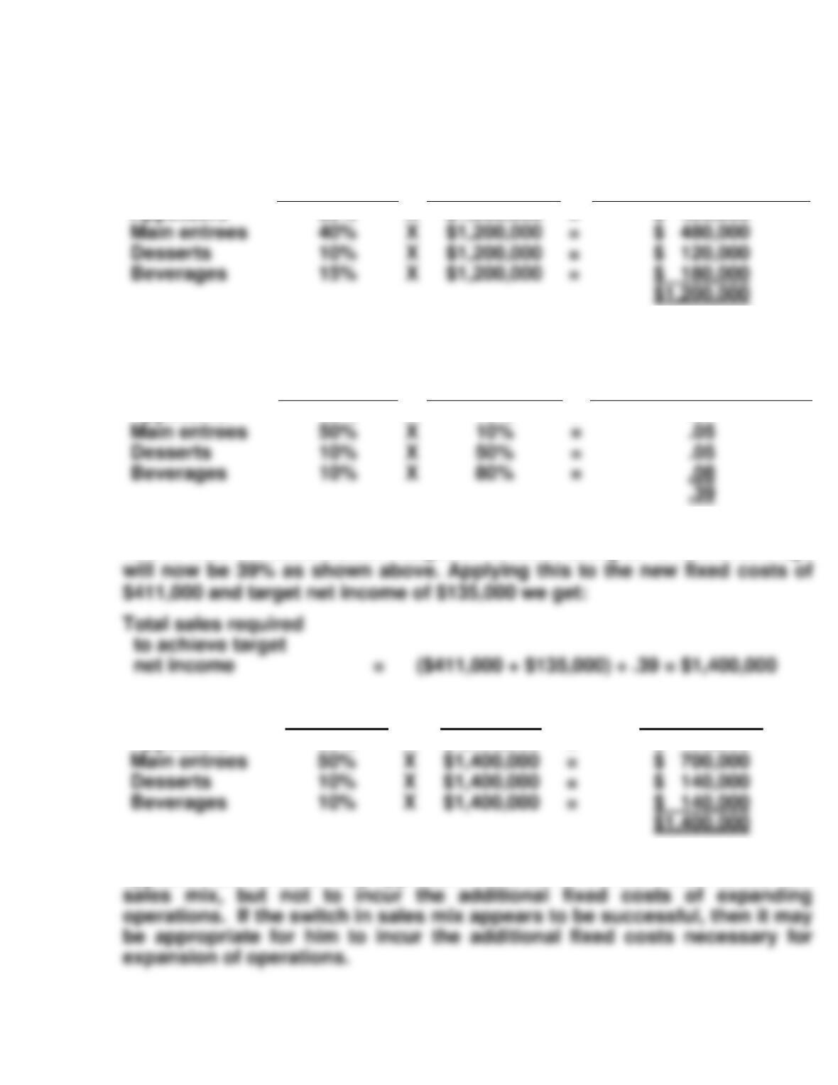
PROBLEM 6-3C (Continued)
Thus, sales would have to increase by $200,000 ($1,200,000 – $1,000,000) to
achieve the target net income. This increase in sales is driven by the
increase in fixed costs. The sales of each product line would be:
Sales Mix
Percentage
X
Total Sales
Needed
=
Sales Dollars
Per Product
Appetizers
35%
X
$1,200,000
=
$ 420,000
(c)
Sales Mix
Percentage
X
Contribution
Margin Ratio
=
Weighted-Average
Contribution
Margin Ratio
Desserts
Beverages
X
X
=
=
Appetizers
30%
X
70%
=
.21
The weighted-average contribution margin ratio computed in part (a) was
43.5%. With the contribution margin on entrees falling to 10%, that average
Sales Mix
Percentage
X
Total Sales
Needed
=
Sales from
Each Product
Beverages
X
=
Appetizers
30%
X
$1,400,000
=
$ 420,000
Relative to parts (a) and (b), the total required sales for (c) would increase. It
appears that the least risky approach would be for Bart to switch to the new
Desserts
Beverages
X
X
=
=
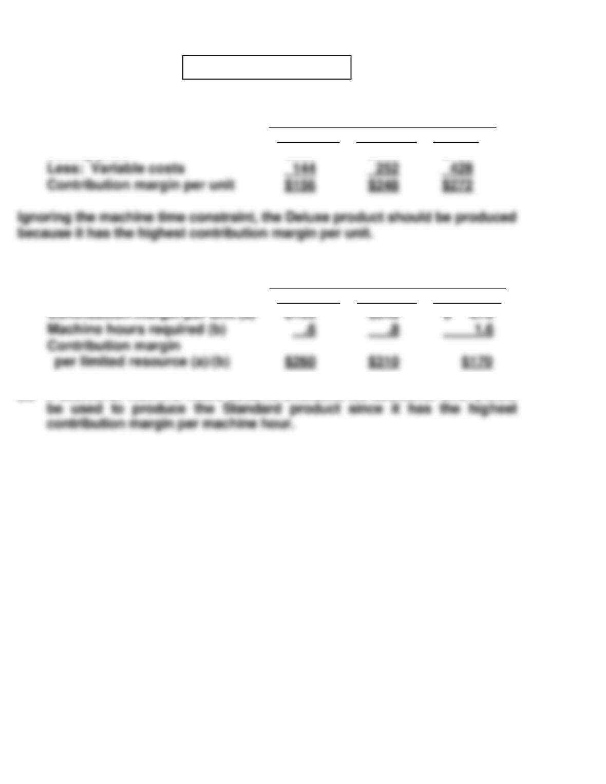
PROBLEM 6-4C
(a)
Product
Economy
Standard
Deluxe
Selling price
$300
$500
$700
(b)
Product
Economy
Standard
Deluxe
(c) If additional machine hours become available, the additional time should
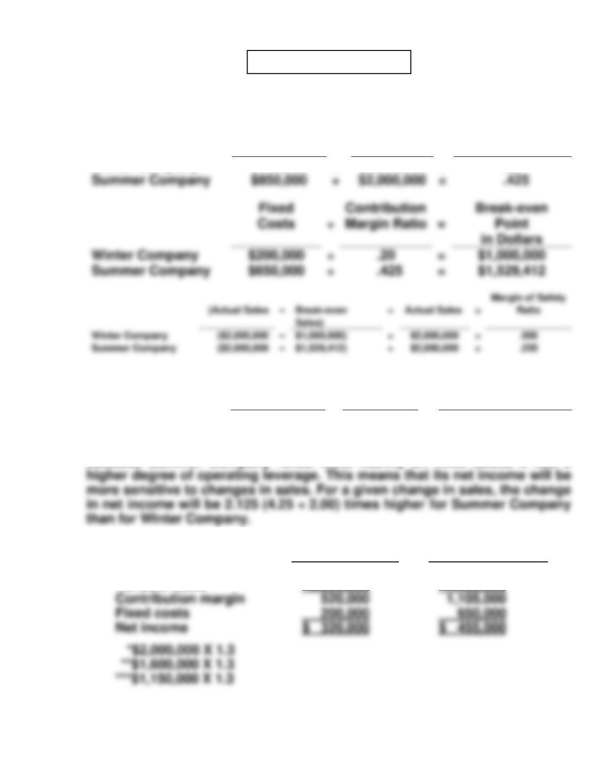
(a) To determine the break-even point in dollars we must first calculate the
contribution margin ratio for each company.
Contribution
Margin
÷
Sales
=
Contribution
Margin Ratio
Winter Company
$400,000
÷
$2,000,000
=
.20
(b)
Contribution
Margin
÷
Net
Income
=
Degree of Operating
Leverage
Winter Company
Summer Company
$400,000
$850,000
÷
÷
$200,000
$200,000
=
=
2.00
4.25
Because Summer Company relies more heavily on fixed costs, it has a
(c)
Winter Company Summer Company
Sales $2,600,000* $2,600,000
Variable costs 2,080,000** 1,495,000***
PROBLEM 6-5C
Summer Company
÷
=
Winter Company
Summer Company
÷
÷
=
=
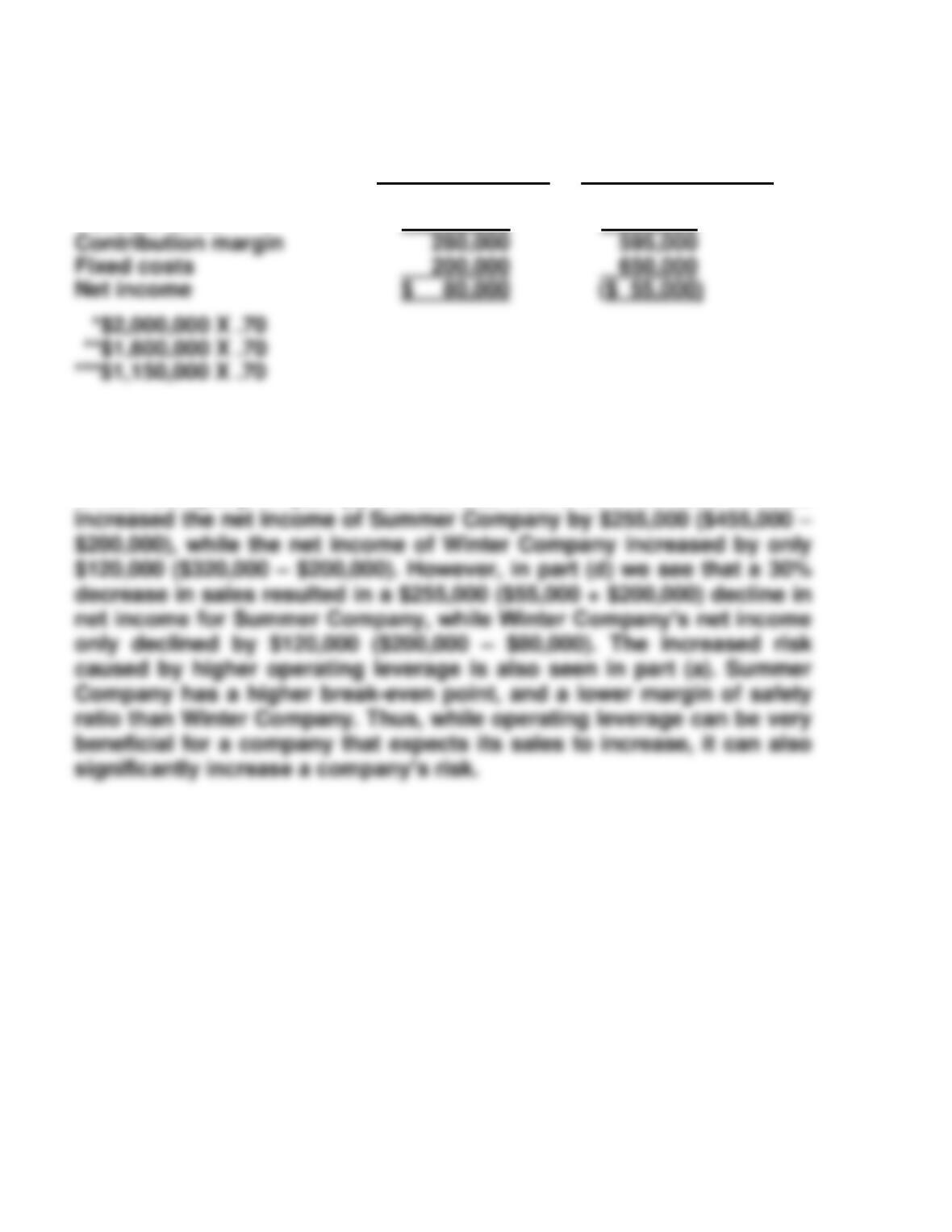
PROBLEM 6-5C (Continued)
(d)
Winter Company Summer Company
Sales $1,400,000* $1,400,000
Variable costs 1,120,000** 805,000***
(e) In part (b) the degree of operating leverage of Summer Company was
higher than that of Winter Company, telling us that the net income of
Summer Company was more sensitive to changes in sales than that of
Winter Company. In part (c) we see that with a 30% increase in sales
PROBLEM 6-6C
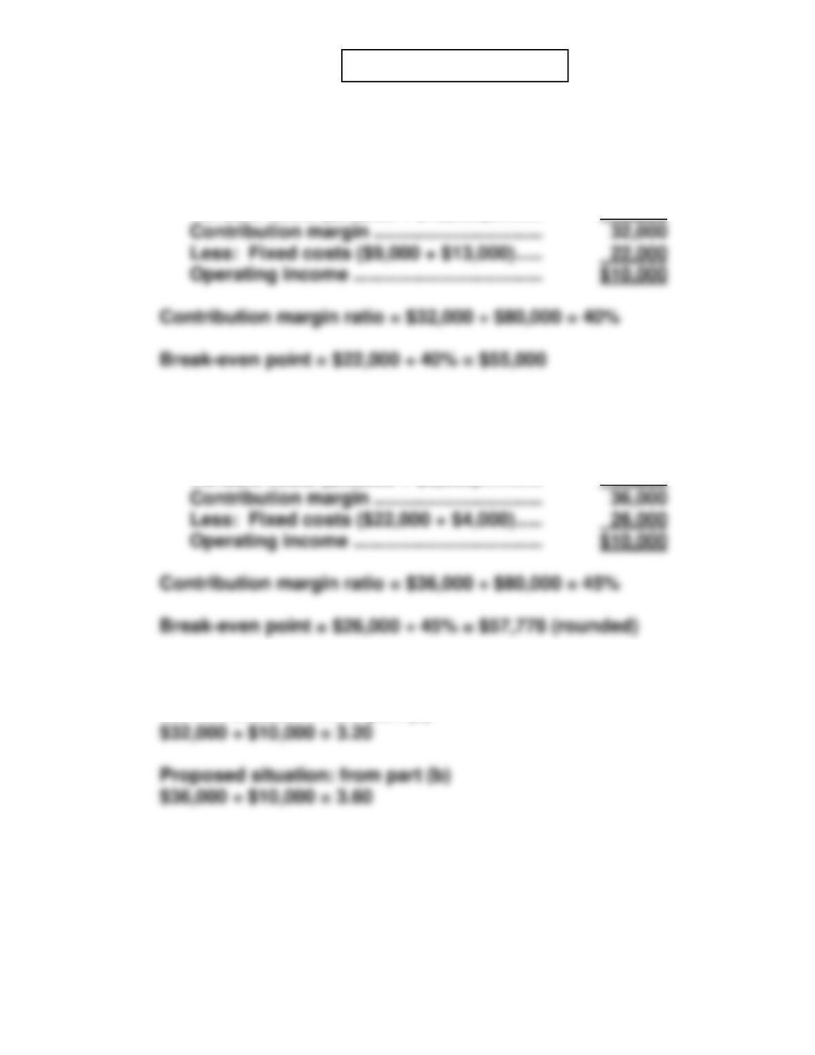
(a) Reformat the income statement to CVP format.
All amount are in $000s.
Sales ………………………………………………… $80,000
Variable costs ($36,000 + $12,000) ………. 48,000
(b) If a hired workforce replaces sales agents, commissions will be reduced
to 10% of sales, or $8,000; but fixed costs will increase by $4,000.
Sales ………………………………………………… $80,000
Variable costs ($36,000 + $8,000) ………… 44,000
(c) Operating leverage = contribution margin ÷ operating income
Current situation: from part (a)
PROBLEM 6-6C (Continued)
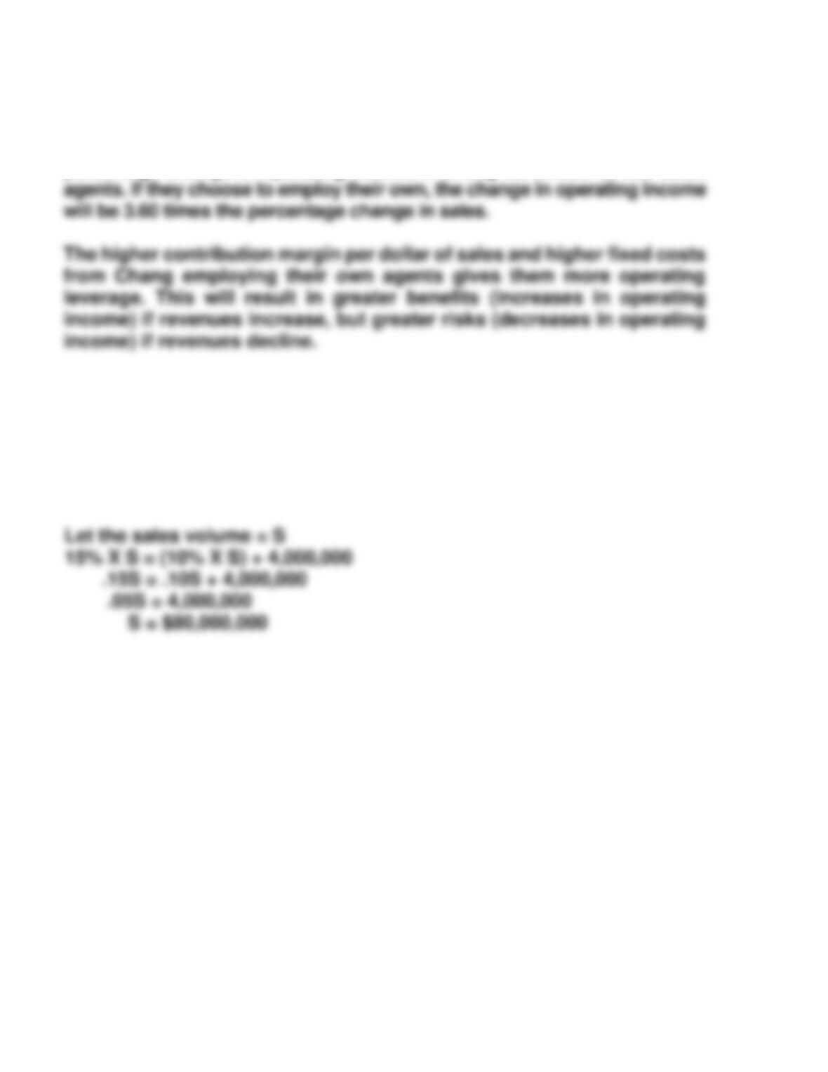
The calculations indicate that at a sales level of $80 million, a percentage
change in sales and contribution margin will result in 3.20 times that
percentage change in operating income if Chang continues to use sales
(d) The sales level at which operating incomes will be identical is called the
point of indifference. This would be when the cost of the network of
agents (15% of sales) is exactly equal to the cost of paying employees
10% commission along with additional fixed costs of $4.0 million. None
of the other costs is relevant, because they will not change between
alternatives.
*PROBLEM 6-7C
(a) PEPPER COMPANY
Income Statement
For the Year Ended December 31, 2016
Variable Costing
Sales (400,000 yards X $3) ………………………
Variable cost of goods sold
Inventory, January 1 ………………………..
Variable cost of goods manufactured
$ –0–
375,000
$1,200,000
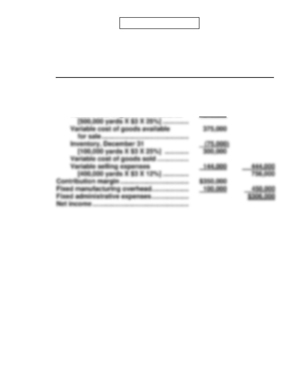
*PROBLEM 6-7C (Continued)
PEPPER COMPANY
Income Statement
For the Year Ended December 31, 2017
Variable Costing
Sales (500,000 tons X $3) …………………………
Variable cost of goods sold
Inventory, January 1 …………………………
Variable cost of goods manufactured
[400,000 tons X ($3 X .25)] ……………..
Variable cost of goods available
$ 75,000
300,000
375,000
$1,500,000
(b) PEPPER COMPANY
Income Statement
For the Year Ended December 31, 2016
Absorption Costing
Sales (400,000 yards X $3) …………………..
Cost of goods sold
Inventory, January 1 …………………….
Cost of goods manufactured…………
–0–
725,000
(1)
$1,200,000
(2) 100,000 X [($3 X 25%) + ($350,000 ÷ 500,000)]
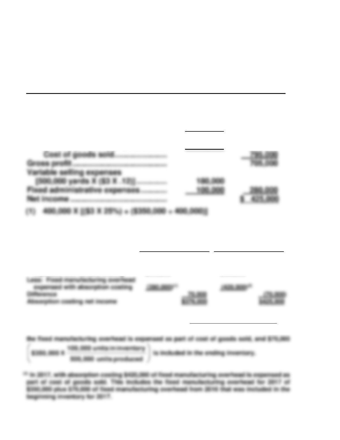
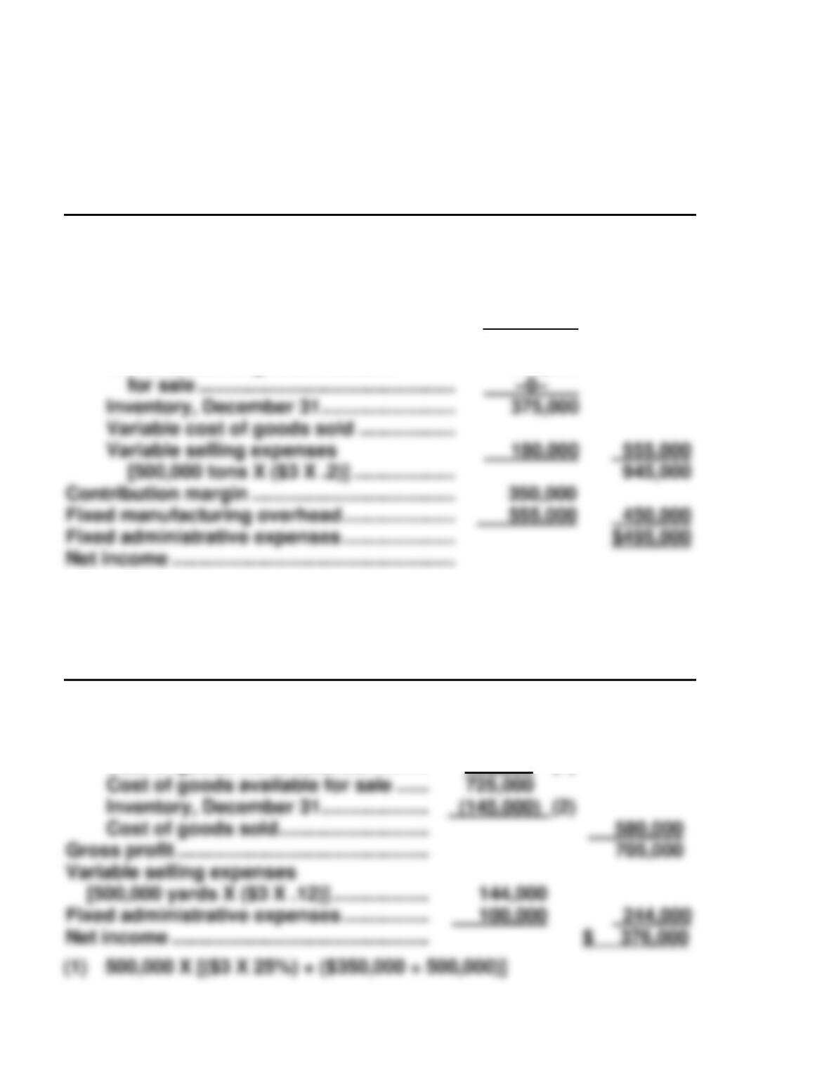
*PROBLEM 6-7C (Continued)
PEPPER COMPANY
Income Statement
For the Year Ended December 31, 2017
Absorption Costing
Sales (500,000 yards X $3) ……………….
Cost of goods sold
Inventory, January 1 …………………
Cost of goods manufactured………
Cost of goods available for sale …
Inventory, December 31 …………….
$ 145,000
650,000
795,000
–0–
(1)
$1,500,000
(c) The variable costing and the absorption costing income from operations
can be reconciled as follows:
2016
2017
Absorption costing net income
Variable costing net income
Fixed manufacturing overhead
expensed with variable costing
$350,000
$306,000
$350,000
$495,000
(1)In 2016, with absorption costing $280,000
400,000 units sold
$350,000 X 500,000 units manufactured
of

*PROBLEM 6-7C (Continued)
(d) Income parallels sales under variable costing as seen in the increase in
net income in 2017 when 100,000 additional units were sold. In contrast,
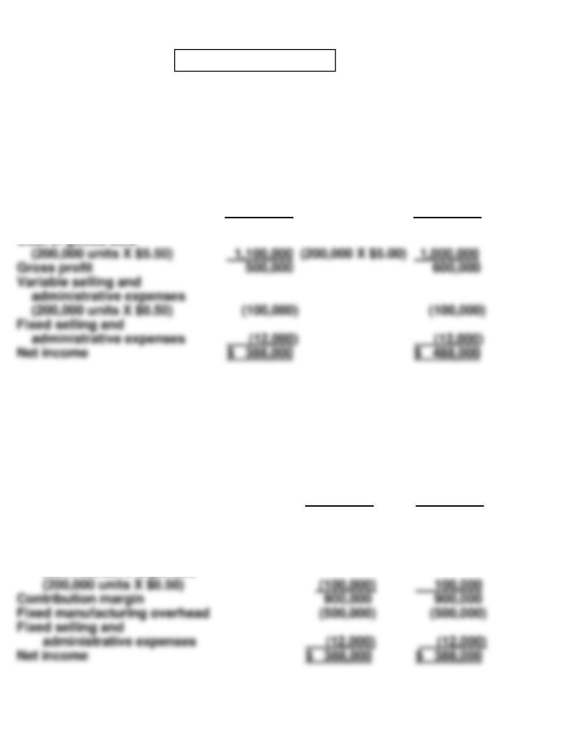
*PROBLEM 6-8C
(a)
SPARK DIVISION
Income Statement
For the Year Ended December 31, 2017
Absorption Costing
_______________________________________________________________
200,000 250,000
Produced Produced
Sales (200,000 units X $8) $1,600,000 $1,600,000
(b)
SPARK DIVISION
Income Statement
For the Year Ended December 31, 2017
Variable Costing
_______________________________________________________________
200,000 250,000
Produced Produced
Sales (200,000 units X $8) $1,600,000 $1,600,000
Variable cost of goods sold
(200,000 units X $3) (600,000) (600,000)
Variable selling and
administrative expenses
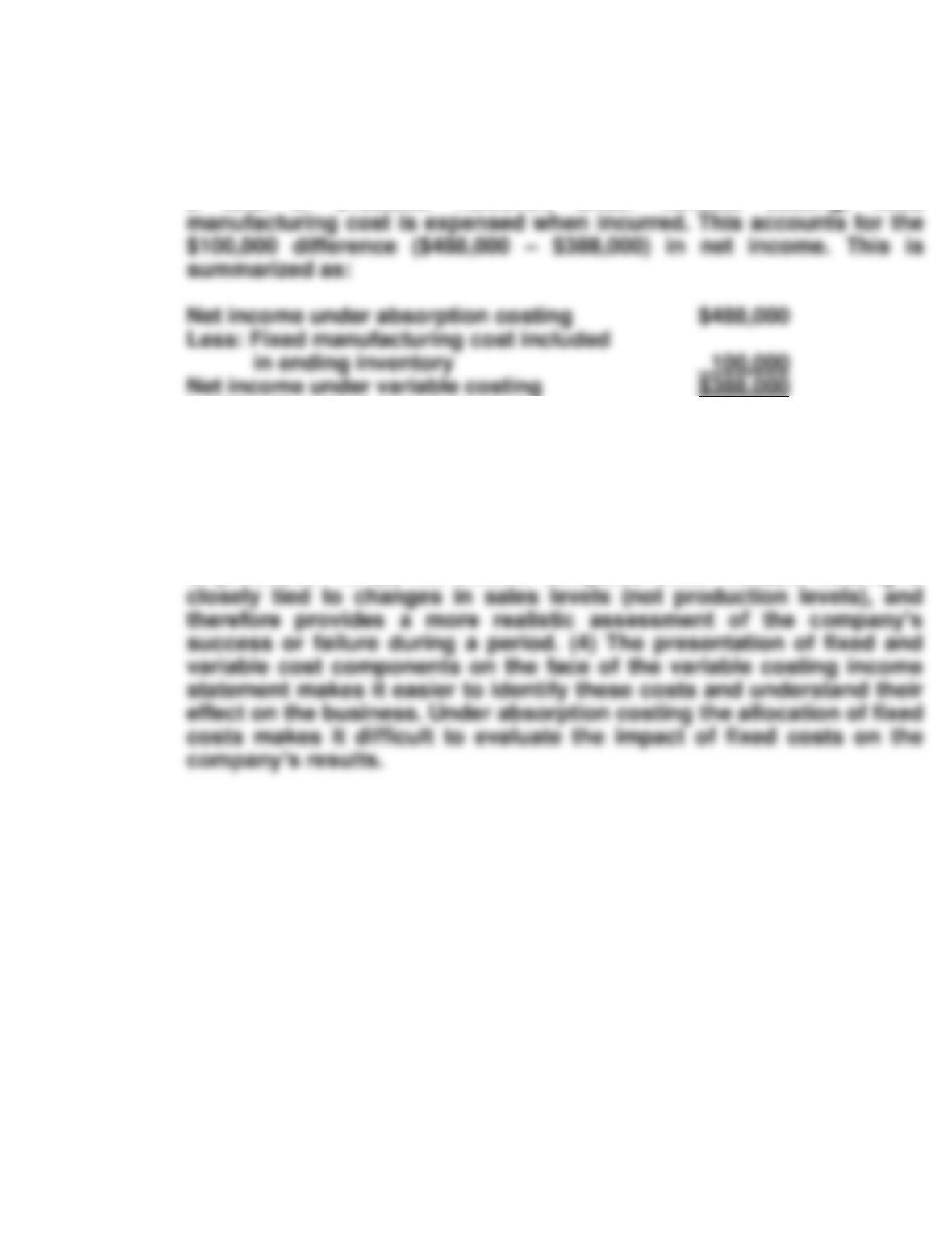
*PROBLEM 6-8C (Continued)
(c) If the company produces 250,000 units, but only sells 200,000 units, then
50,000 units will remain in ending inventory. Under absorption costing
these 50,000 units will each include $2.00 of fixed manufacturing cost—
a total of $100,000. However, under variable costing, fixed
(d) Variable costing has a number of advantages over absorption costing
for decision making and evaluation purposes. (1) The use of variable
costing is consistent with cost-volume-profit and incremental analysis:
(2) Net income computed under variable costing is unaffected by
changes in production levels. Note that in our example, under variable
costing the company’s net income is $388,000 no matter what the level
of production is. (3) Net income computed under variable costing is