PROBLEM 6-2C
(a)
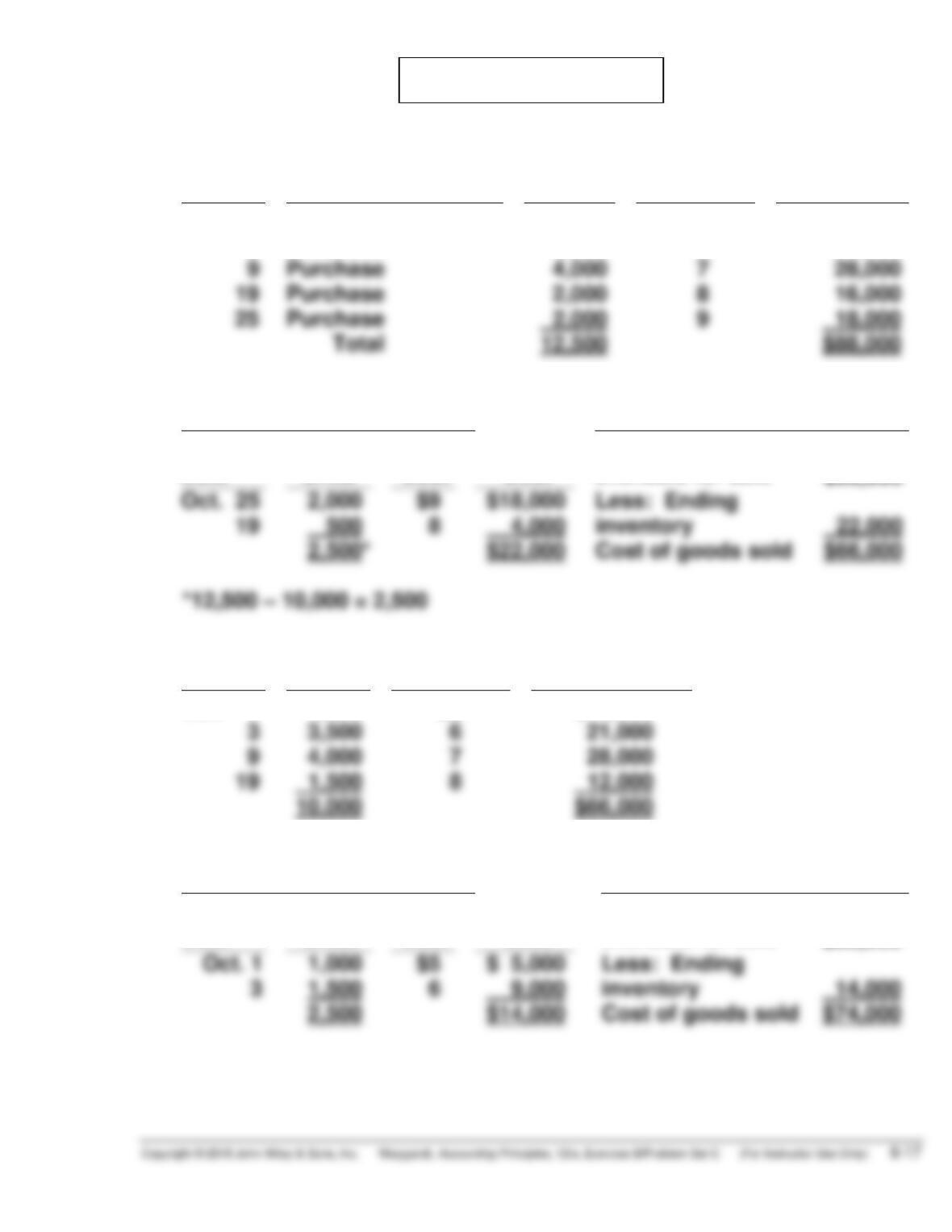
COST OF GOODS AVAILABLE FOR SALE
Date
Explanation
Units
Unit Cost
Total Cost
Oct. 1
Beginning Inventory
1,000
$5
$ 5,000
3
Purchase
3,500
6
21,000
9
Purchase
4,000
7
28,000
Purchase
2,000
Purchase
9
(b)
FIFO
(1)
Ending Inventory
(2)
Cost of Goods Sold
Date
Units
Unit
Cost
Total
Cost
Cost of goods
available for sale
$88,000
2,000
500
8
4,000
2,500*
$22,000
Cost of goods sold
$66,000
Proof of Cost of Goods Sold
Date
Units
Unit Cost
Total Cost
Oct. 1
1,000
$5
$ 5,000
3
3,500
6
21,000
9
4,000
7
8
10,000
$66,000
LIFO
(1)
Ending Inventory
(2)
Cost of Goods Sold
Date
Units
Unit
Cost
Total
Cost
Cost of goods
available for sale
$88,000
1,000
$ 5,000
3
1,500
6
9,000
2,500
$14,000
Cost of goods sold
PROBLEM 6-2C (Continued)
Proof of Cost of Goods Sold
Date
Units
Unit
Cost
Total
Cost
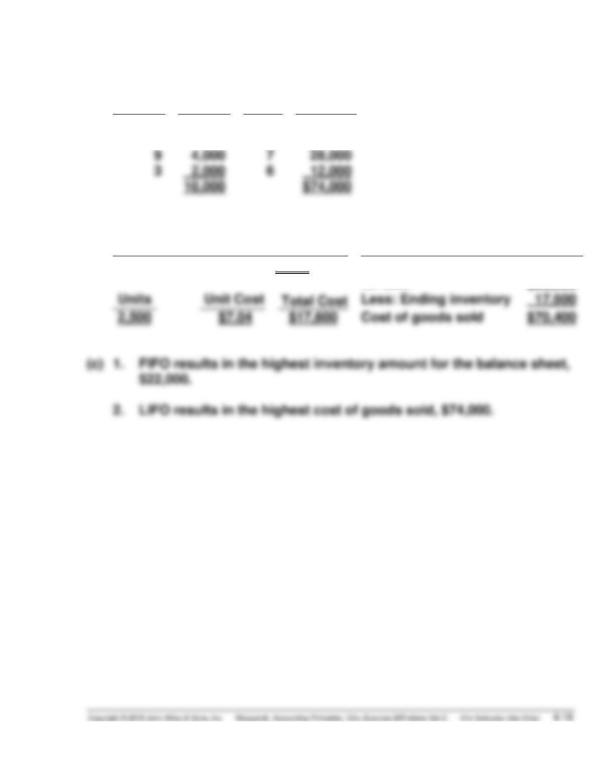
Oct. 25
2,000
$9
$18,000
19
2,000
8
16,000
9
4,000
7
28,000
3
6
12,000
10,000
$74,000
AVERAGE COST
(1)
Ending Inventory
(2)
Cost of Goods Sold
$88,000 ÷ 12,500 = $7.04
Cost of goods available
for sale
$88,000
Total Cost
Cost of goods sold
(c) 1. FIFO results in the highest inventory amount for the balance sheet,
$22,000.
PROBLEM 6-3C
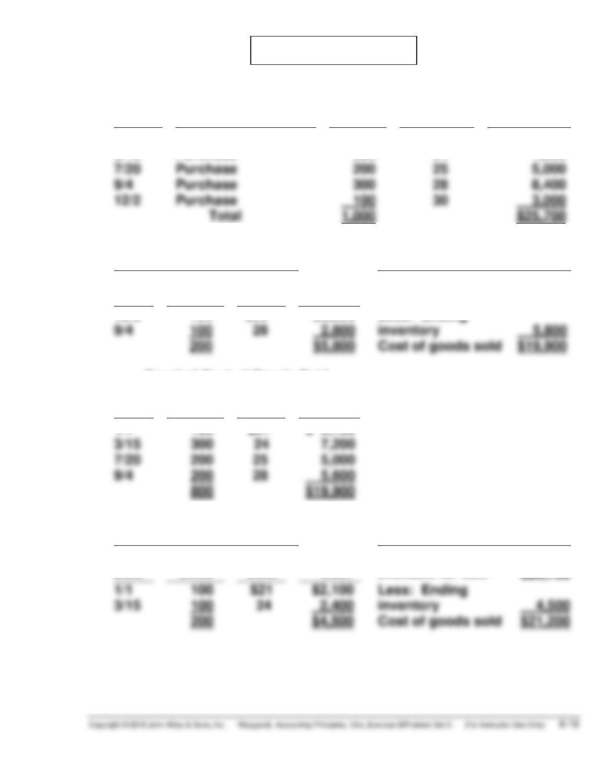
(a)
COST OF GOODS AVAILABLE FOR SALE
Date
Explanation
Units
Unit Cost
Total Cost
1/1
Beginning Inventory
100
$21
$ 2,100
3/15
Purchase
300
24
7,200
7/20
Purchase
200
25
5,000
9/4
Purchase
300
12/2
Purchase
30
(b)
FIFO
(1)
Ending Inventory
(2)
Cost of Goods Sold
Date
Units
Unit
Cost
Total
Cost
Cost of goods
available for sale
$25,700
12/2
100
$30
$3,000
9/4
100
Cost of goods sold
$19,900
Less: Ending
Proof of Cost of Goods Sold
Date
Units
Unit
Cost
Total
Cost
1/1
100
$21
$ 2,100
3/15
300
24
7,200
7/20
200
9/4
200
800
(c)
LIFO
(1)
Ending Inventory
(2)
Cost of Goods Sold
Date
Units
Unit
Cost
Total
Cost
Cost of goods
available for sale
1/1
100
$2,100
Less: Ending
3/15
100
200
Cost of goods sold
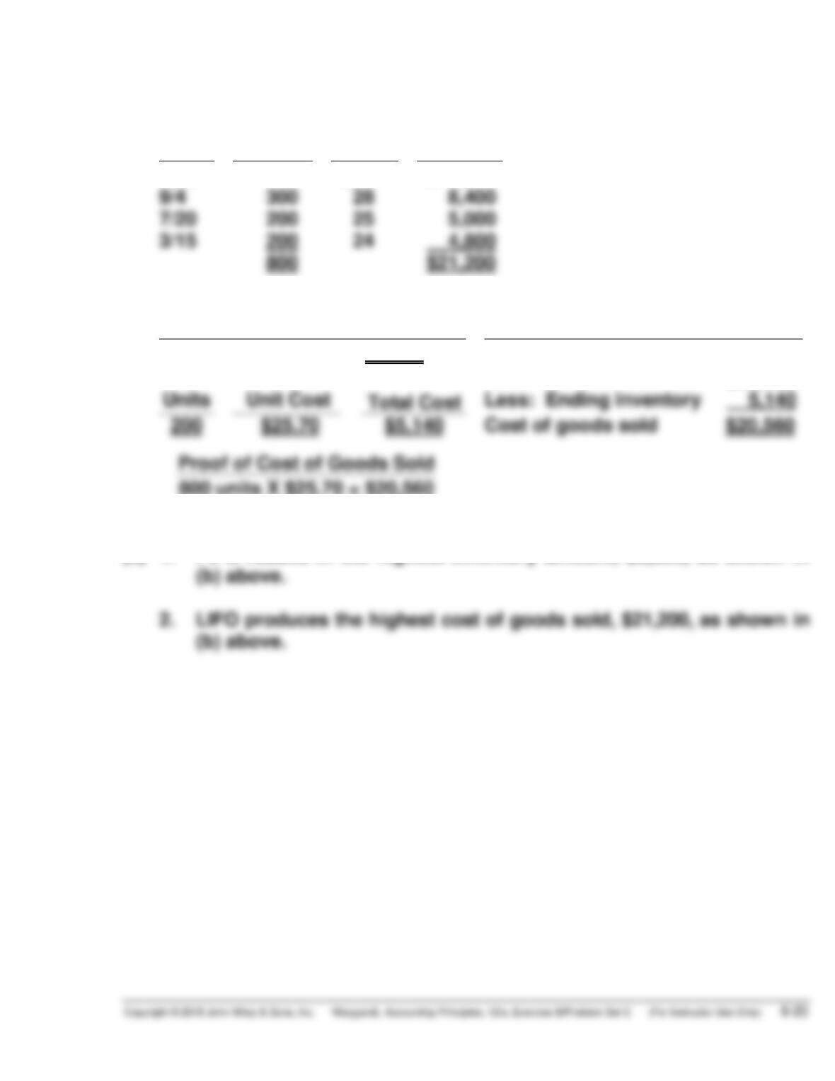
PROBLEM 6-3C (Continued)
Proof of Cost of Goods Sold
Date
Units
Unit
Cost
Total
Cost
12/2
100
$30
$ 3,000
9/4
7/20
3/15
200
4,800
$21,200
AVERAGE COST
(1)
Ending Inventory
(2)
Cost of Goods Sold
$25,700 ÷ 1,000 = $25.70
Cost of goods available
for sale
$25,700
Cost of goods sold
$20,560
Proof of Cost of Goods Sold
800 units X $25.70 = $20,560
(c) 1. FIFO results in the highest inventory amount, $5,800, as shown in
(b) above.
PROBLEM 6-4C
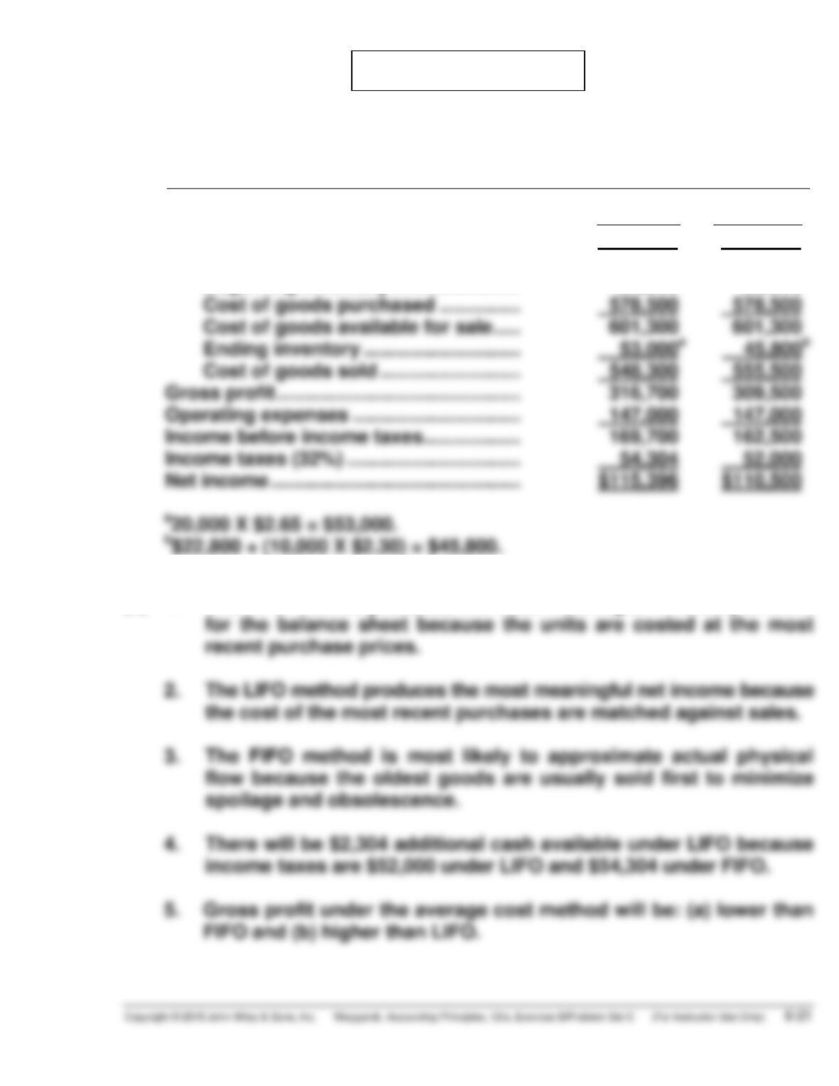
(a) MATHENY INC.
Condensed Income Statements
For the Year Ended December 31, 2017
FIFO
LIFO
Sales ……………………………………………….. $865,000 $865,000
Cost of goods sold
Beginning inventory …………………… 22,800 22,800
Cost of goods purchased …………… 578,500 578,500
Cost of goods available for sale ….. 601,300 601,300
(b) 1. The FIFO method produces the most meaningful inventory amount
for the balance sheet because the units are costed at the most
recent purchase prices.
PROBLEM 6-5C
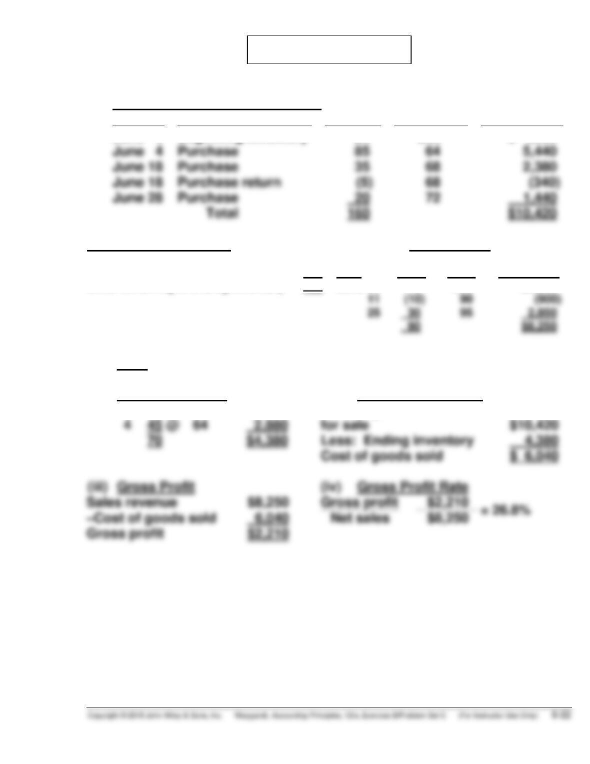
(a)
Cost of Goods Available for Sale
Date
Explanation
Units
Unit Cost
Total Cost
June 1
Beginning Inventory
25
$60
$ 1,500
June 4
Purchase
85
64
5,440
June 18
Purchase
35
68
June 18
Purchase return
(340)
June 28
Purchase
72
1,440
Ending Inventory in Units:
Sales Revenue
Units available for sale
160
Unit
—Sales (70 – 10 + 30)
90
Date
Units
Price
Total Sales
Units remaining in ending inventory
70
June 10
70
$90
$6,300
(10)
2,850
(1)
LIFO
(i)
Ending Inventory
(ii)
Cost of Goods Sold
Less: Ending inventory
Cost of goods sold
(iii)
Gross Profit
(iv)
Gross Profit Rate
Sales revenue
Gross profit
$8,250
Gross profit
June 1
25 @ $60
$1,500
Cost of goods available
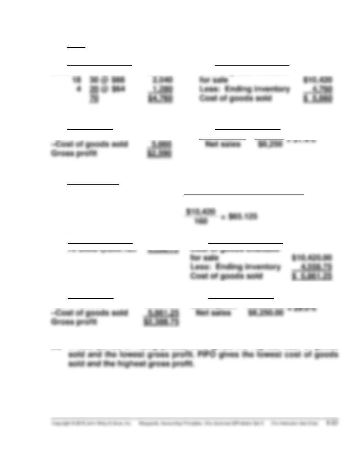
PROBLEM 6-5C (Continued)
(2)
FIFO
(i)
Ending Inventory
(ii)
Cost of Goods Sold
June 28
18
20 @ $72
30 @ $68
$1,440
2,040
Cost of goods available
for sale
$10,420
Less: Ending inventory
Cost of goods sold
(iii)
Gross Profit
(iv)
Gross Profit Rate
Sales revenue
$8,250
Gross profit
$2,590
$8,250
Gross profit
$2,590
(3)
Average-Cost
Weighted-average cost per unit:
Cost of goods available for sale
Units available for sale
(i)
Ending Inventory
(ii)
Cost of Goods Sold
70 units @$65.125
4,558.75
Cost of goods available
for sale
$10,420.00
Less: Ending inventory
4,558.75
Cost of goods sold
$ 5,861.25
(iii)
Gross Profit
(iv)
Gross Profit Rate
Sales revenue
$8,250.00
Gross profit
$2,388.75
Net sales
$8,250.00
Gross profit
(b) In this period of rising prices, LIFO gives the highest cost of goods
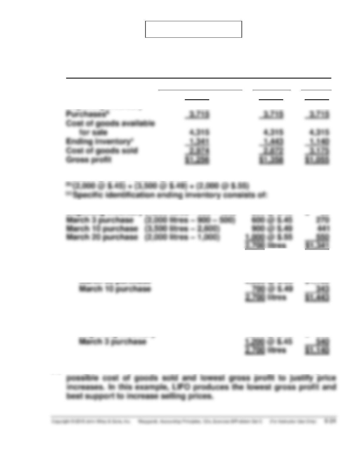
PROBLEM 6-6C
(a) WAINWRIGHT INC.
Income Statement (partial)
For the Year Ended March 31, 2017
Specific Identification
FIFO
LIFO
Sales revenuea
$4,230
$4,230
$4,230
Beginning inventory
600
600
600
Cost of goods sold
Gross profit
(a) (1,800 @ $.60) + (4,500 @ $.70)
Beginning inventory (1,500 litres – 900 – 400)
200 @ $.40
$ 80
March 3 purchase (2,000 litres – 900 – 500)
600 @ $.45
270
March 10 purchase (3,500 litres – 2,600)
900 @ $.49
March 20 purchase (2,000 litres – 1,000)
1,000 @ $.55
550
FIFO ending inventory consists of:
March 20 purchase
$1,100
March 10 purchase
343
LIFO ending inventory consists of:
Beginning inventory
1,500 @ $.40
$ 600
March 3 purchase
1,200 @ $.45
540
(b) Companies can choose a cost flow method that produces the highest
PROBLEM 6-7C
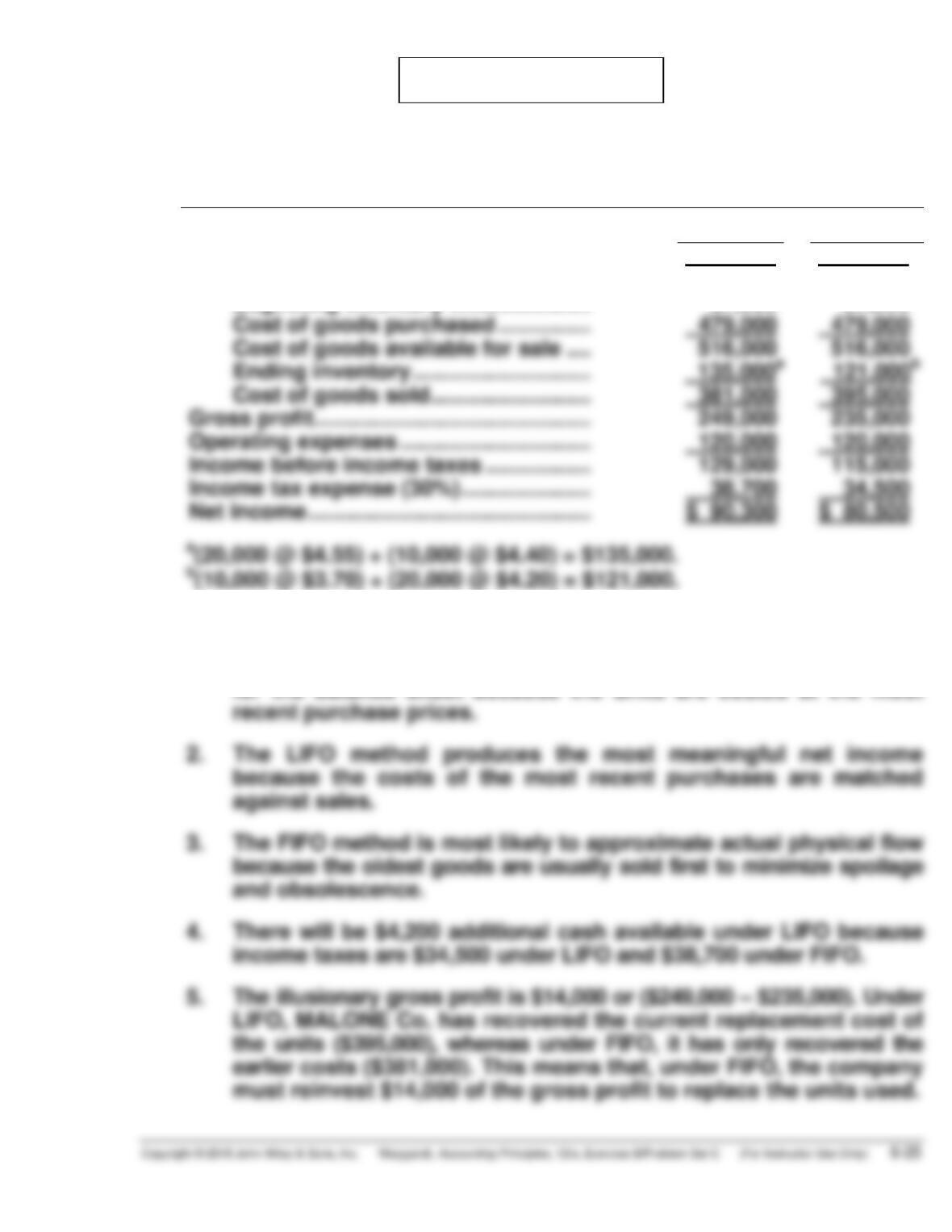
(a) MALONE CO.
Condensed Income Statement
For the Year Ended December 31, 2017
FIFO
LIFO
Sales ……………………………………………….. $630,000 $630,000
Cost of goods sold
Beginning inventory ………………….. 37,000 37,000
Cost of goods purchased …………… 479,000 479,000
(b) Answers to questions:
1. The FIFO method produces the most meaningful inventory amount
for the balance sheet because the units are costed at the most
recent purchase prices.
2. The LIFO method produces the most meaningful net income
because the costs of the most recent purchases are matched
against sales.
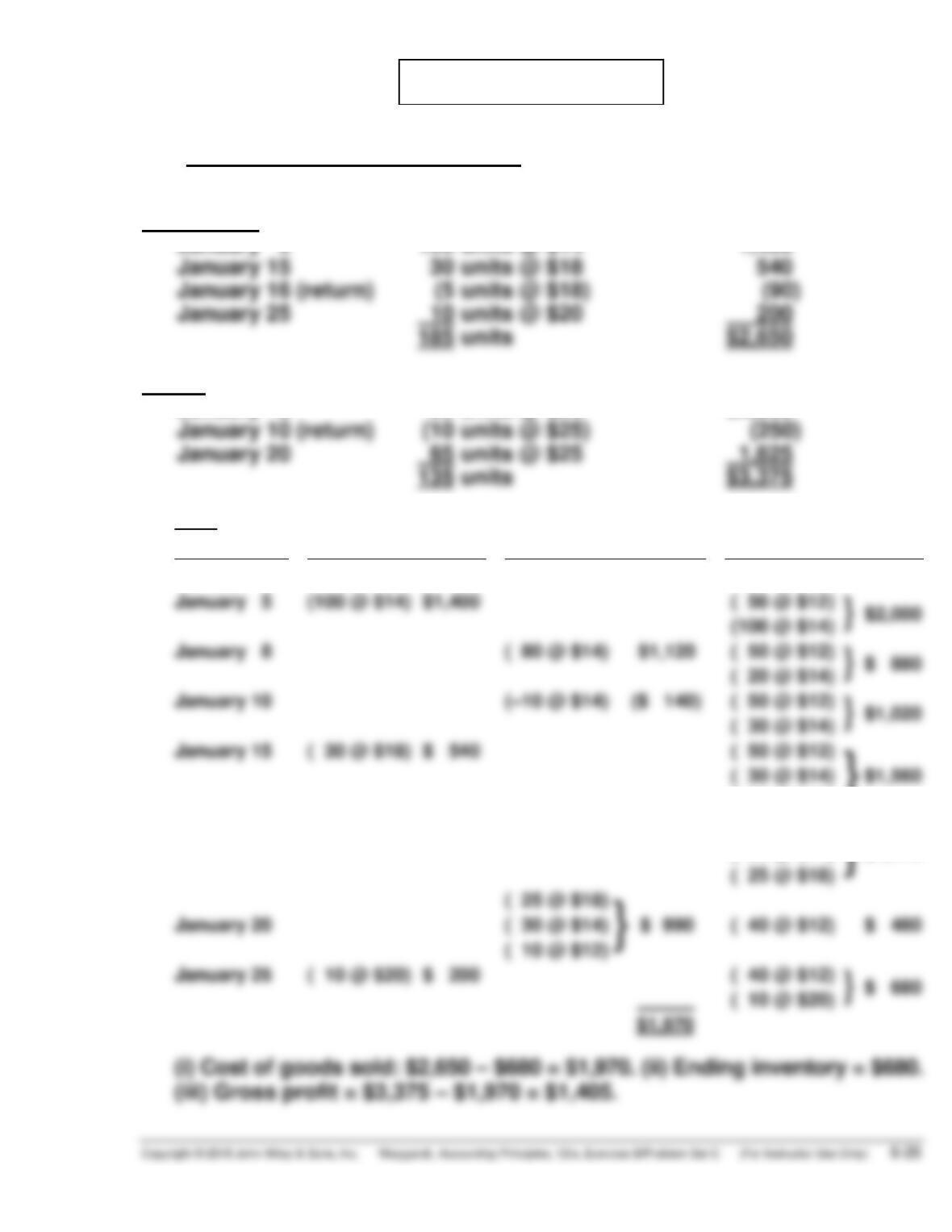
*PROBLEM 6-8C
(a) Cost of goods available for sale:
Inventory
50 units @ $12
$ 600
Purchases:
January 5
100 units @ $14
1,400
January 15
30 units @ $18
January 16 (return)
January 25
10 units @ $20
200
185 units
$2,650
Sales:
January 8
80 units @ $25
$2,000
January 10 (return)
(10 units @ $25)
January 20
65 units @ $25
135 units
$3,375
(1)
LIFO
Date
Purchases
Cost of Goods Sold
Balance
January 1
( 50 @ $12)
$ 600
January 5
(100 @ $14) $1,400
( 50 @ $12)
}
$2,000
(100 @ $14)
January 8
( 80 @ $14) $1,120
( 50 @ $12)
$ 880
( 20 @ $14)
January 10
( 50 @ $12)
$1,020
( 30 @ $14)
January 15
( 30 @ $18) $ 540
( 50 @ $12)
$1,560
( 30 @ $14)
}
( 30 @ $18)
January 16
( –5 @ $18) ($ 90)
( 50 @ $12)
}
$1,470
( 30 @ $14)
( 25 @ $18)
( 25 @ $18)
January 20
( 30 @ $14)
( 40 @ $12)
$ 480
( 10 @ $12)
January 25
( 10 @ $20) $ 200
( 40 @ $12)
$ 680
( 10 @ $20)
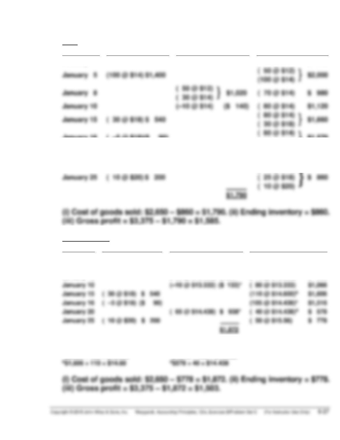
*PROBLEM 6-8C (Continued)
(2)
FIFO
Date
Purchases
Cost of Goods Sold
Balance
January 1
( 50 @ $12)
$ 600
January 5
(100 @ $14) $1,400
( 50 @ $12)
}
$2,000
(100 @ $14)
January 8
$1,020
$ 980
( 30 @ $14)
( 80 @ $14)
$1,120
January 15
( 30 @ $18) $ 540
( 80 @ $14)
}
$1,660
( 30 @ $18)
( 80 @ $14)
( 25 @ $18)
January 20
(65 @ $14)
$ 910
( 15 @ $14)
( 25 @ $18)
}
$ 660
( 10 @ $20)
( 15 @ $14)
(3)
Moving-Average
Date
Purchases
Cost of Goods Sold
Balance
January 1
( 50 @ $12)
$ 600
January 5
(100 @ $14) $1,400
(150 @ $13.333)a
$2,000
January 8
( 80 @ $13.333)
$1,067*
( 70 @ $13.333)
$ 933
January 10
(–10 @ $13.333)
($ 133)*
( 80 @ $13.333)
$1,066
January 15
( 30 @ $18) $ 540
$1,606
January 16
( –5 @ $18) ($ 90)
$1,516
January 20
( 65 @ $14.438)
$ 938*
$ 578
January 25
( 10 @ $20) $ 200
( 50 @ $15.56)
$ 778
*rounded
a$2,000 ÷ 150 = $13.333 c$1,516 ÷ 105 = $14.438
b$1,606 ÷ 110 = $14.60 d$578 ÷ 40 = $14.438
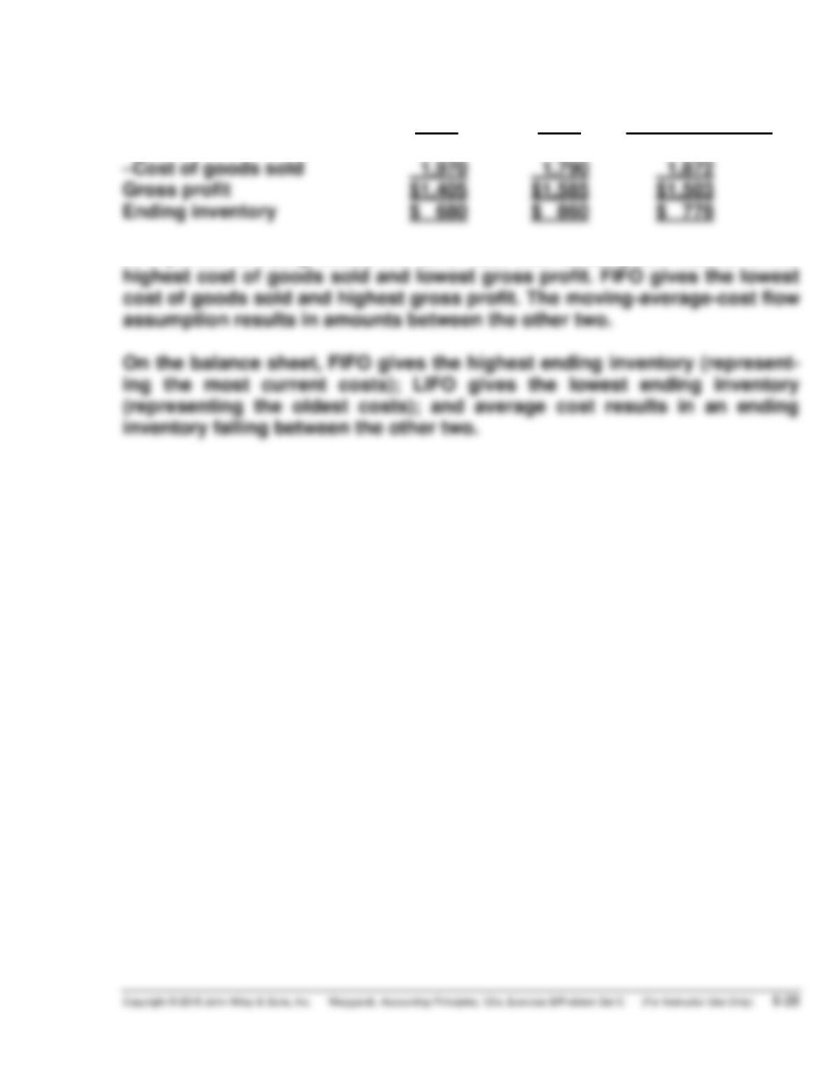
*PROBLEM 6-8C (Continued)
(b)
Gross profit:
LIFO
FIFO
Moving-Average
Sales
$3,375
$3,375
$3,375
Gross profit
$1,405
$1,585
$1,503
In a period of rising costs, the LIFO cost flow assumption results in the
highest cost of goods sold and lowest gross profit. FIFO gives the lowest
cost of goods sold and highest gross profit. The moving-average-cost flow
assumption results in amounts between the other two.
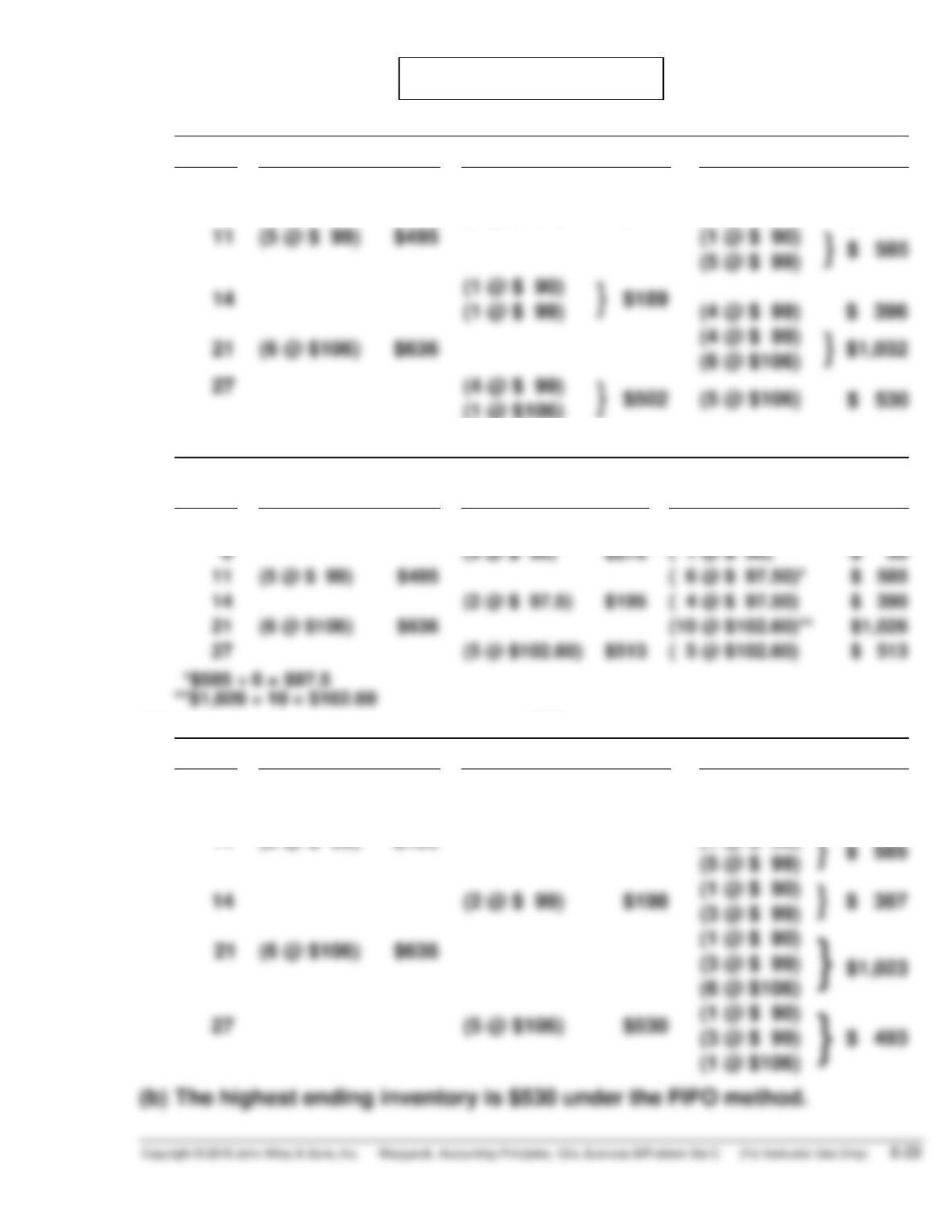
*PROBLEM 6-9C
(1)
FIFO
Date
Purchases
Cost of Goods Sold
Balance
July 1
(4 @ $ 90)
$360
(4 @ $ 90)
$ 360
6
(3 @ $ 90)
$270
(1 @ $ 90)
$ 90
11
(5 @ $ 99)
$495
(1 @ $ 90)
}
$ 585
(5 @ $ 99)
(1 @ $ 90)
(1 @ $ 99)
(4 @ $ 99)
$ 396
(4 @ $ 99)
(6 @ $106)
27
(2)
AVERAGE-COST
Date
Purchases
Cost of
Goods Sold
Balance
July 1
(4 @ $ 90)
$360
( 4 @ $ 90)
$ 360
6
(3 @ $ 90)
$270
( 1 @ $ 90)
$ 90
(5 @ $ 99)
$495
( 6 @ $ 97.50)*
$ 585
(2 @ $ 97.5)
( 4 @ $ 97.50)
$ 390
(6 @ $106)
(10 @ $102.60)**
$1,026
(5 @ $102.60)
( 5 @ $102.60)
$ 513
(3)
LIFO
Date
Purchases
Cost of Goods Sold
Balance
July 1
(4 @ $ 90)
$360
(4 @ $ 90)
$ 360
6
(3 @ $ 90)
$270
(1 @ $ 90)
$ 90
11
(5 @ $ 99)
$495
(1 @ $ 90)
}
$ 585
(5 @ $ 99)
(1 @ $ 90)
(3 @ $ 99)
(1 @ $ 90)
(3 @ $ 99)
(6 @ $106)
(1 @ $ 90)
(3 @ $ 99)
(1 @ $106)
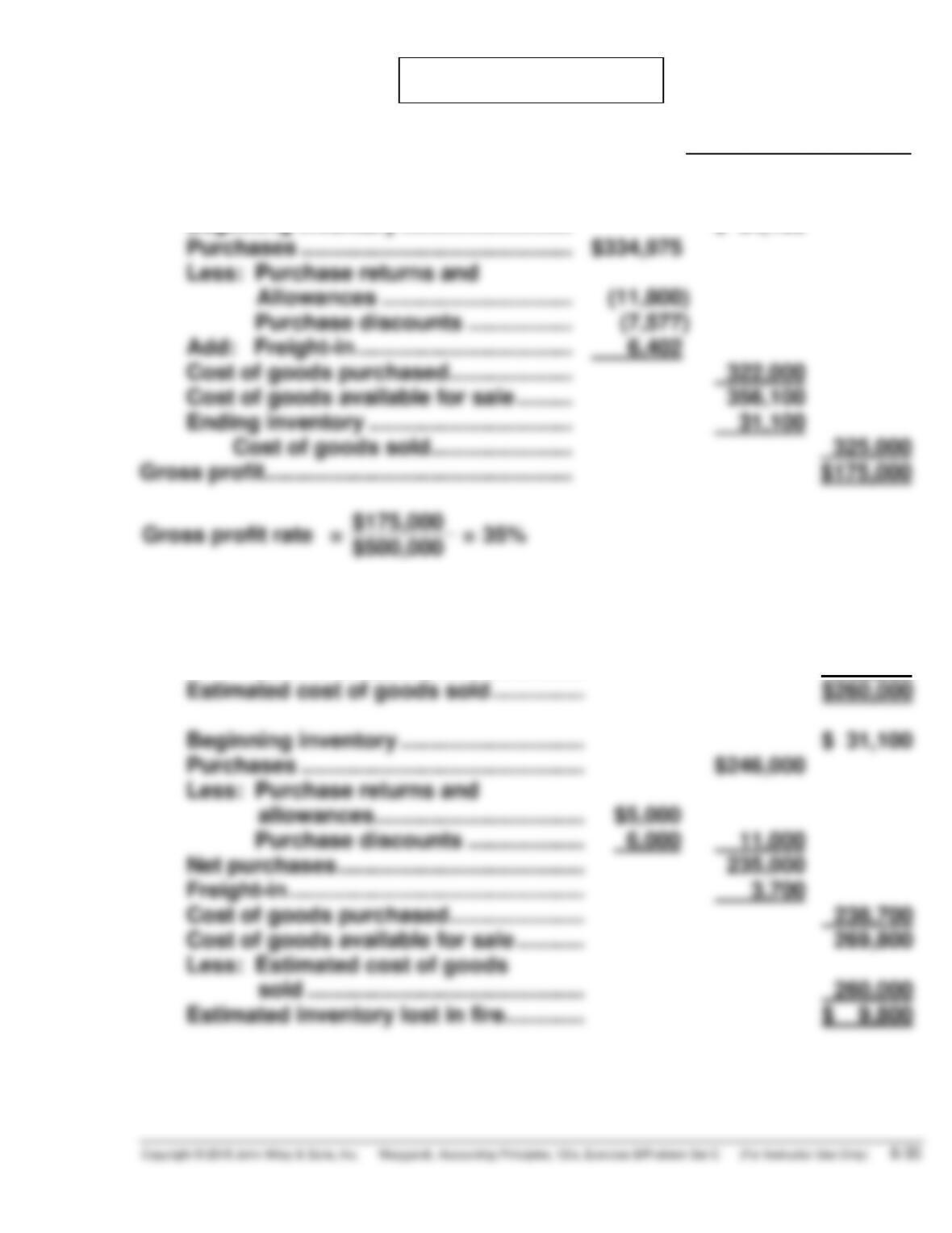
*PROBLEM 6-10C
(a)
November
Net sales ……………………………………………… $500,000
Cost of goods sold
Beginning inventory ………………………. $ 34,100
Purchases …………………………………….. $334,975
Less: Purchase returns and
(b) Net sales ………………………………………… $400,000
Less: Estimated gross profit
(35% X $400,000) …………………… 140,000
Estimated cost of goods sold …………… $260,000
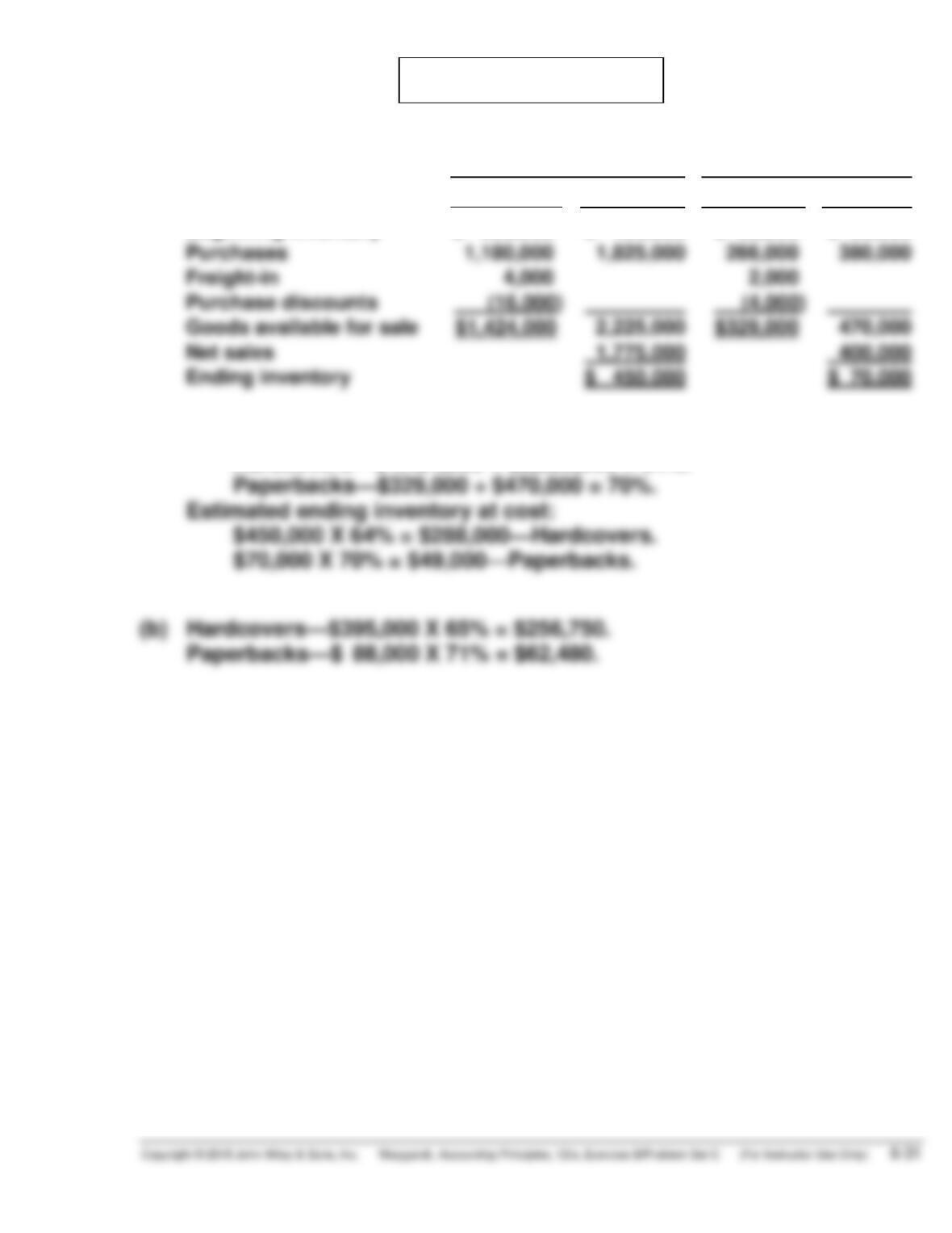
*PROBLEM 6-11C
(a)
Hardcovers
Paperbacks
Cost
Retail
Cost
Retail
Beginning inventory
$ 256,000
$ 400,000
$ 65,000
$ 90,000
Purchases
1,180,000
1,825,000
266,000
380,000
Purchase discounts
Goods available for sale
2,225,000
470,000
Net sales
$ 450,000
$ 70,000
Cost-to-retail ratio:
Hardcovers—$1,424,000 ÷ $2,225,000 = 64%.
Paperbacks—$329,000 ÷ $470,000 = 70%.