CHAPTER 5/CONTINUOUS PROBABILITY DISTRIBUTIONS 79
5.65 If X = change in diastolic blood pressure for a treated patient, then . We have
5.66 If Y = change in diastolic blood pressure for an untreated patient, then . We have
5.67 Suppose we take nreplicate measurements at both baseline and follow-up. In this case,
or
XN n~,533
YN n~,233
80 CHAPTER 5/CONTINUOUS PROBABILITY DISTRIBUTIONS
5.68 The distribution of change in bone mineral density in the placebo group
D
1
is normal with mean
percent and standard deviation = 4.3 percent. We wish to compute
5.69 The distribution of change in bone mineral density in the Alendronate 5 mg group
D
2
is normal with
mean = + 3.5 percent and standard deviation = 4.2 percent. We wish to compute
5.70 Let C = the event that women in the Alendronate 5 mg group are compliers. From the total probability
18.
CHAPTER 5/CONTINUOUS PROBABILITY DISTRIBUTIONS 81
5.71 We wish to compute where X = SBP for 50 year old women. X is assumed to follow a
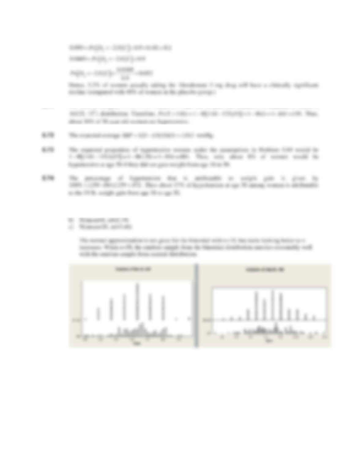
5.75-77 For this exercise, the corresponding normal distributions are
a) N(mean=4, sd=1.55)
Pr
Xt
140
82 CHAPTER 5/CONTINUOUS PROBABILITY DISTRIBUTIONS
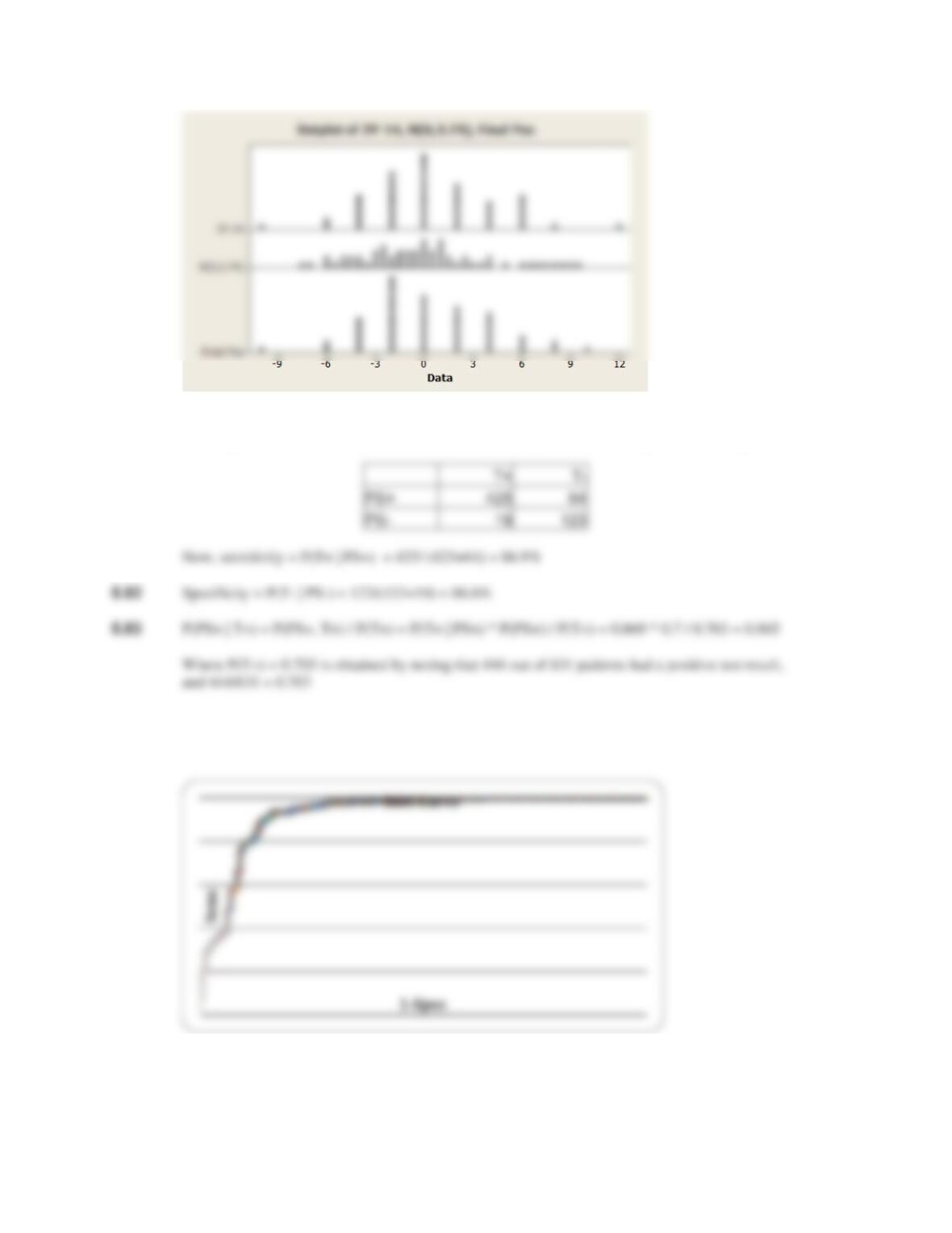
5.78 In this scenario, each ball starts at 0, and has 14 opportunities to move to the right or left by one unit,
with each event occurring with 50% probability. The range of final positions for each ball is [-14, 14].
5.79 If Y~Binomial(n=14, p=0.5), then we can use a normal approximation with mean = 14*0.5 = 7, and
5.80
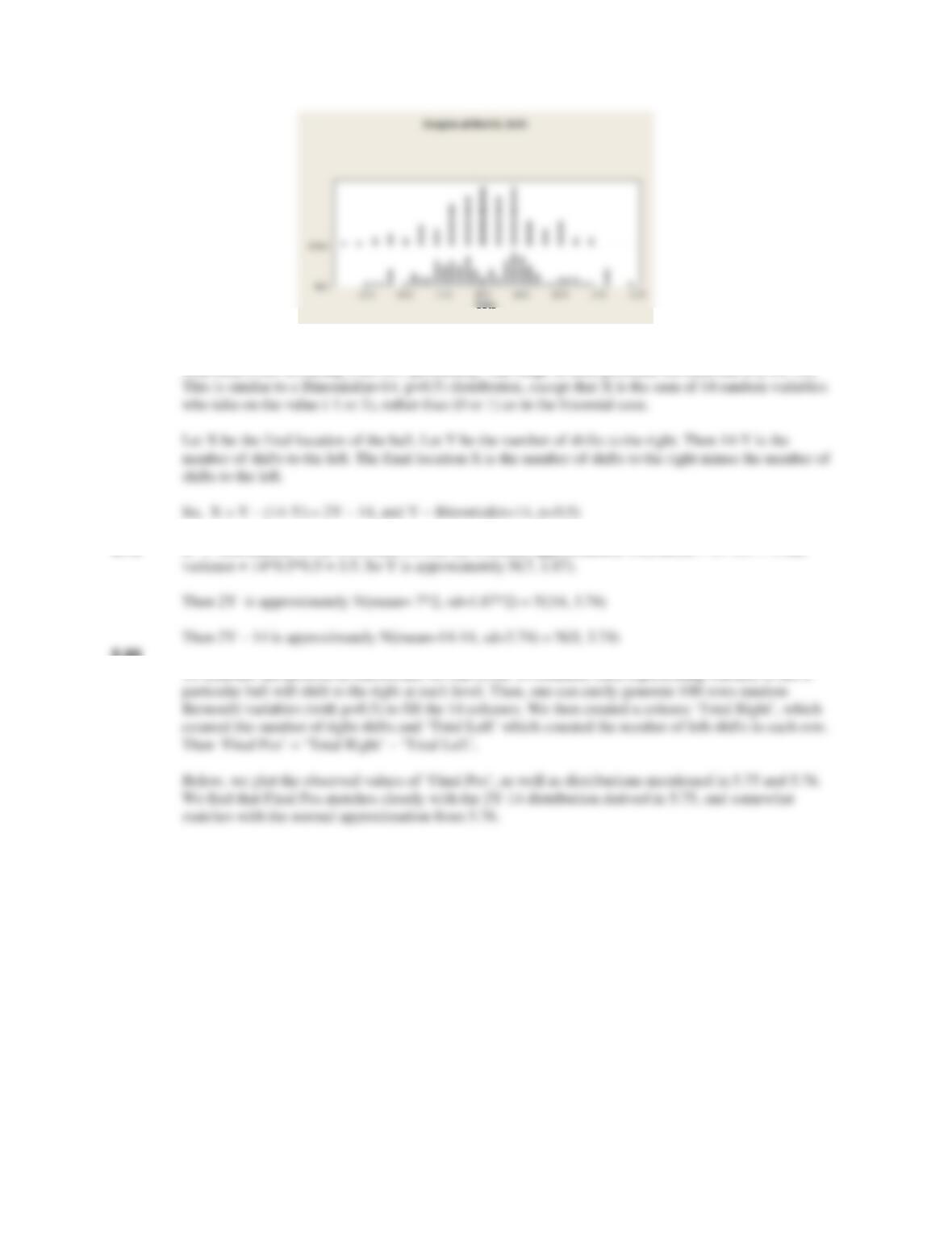
To simulate this process in MINITAB, we can create 14 columns, each representing whether or not a
CHAPTER 5/CONTINUOUS PROBABILITY DISTRIBUTIONS 83
5.81 Defining T+ to mean (maxchg 1.86) and PS+ to mean (piriform=2), we get the following table.
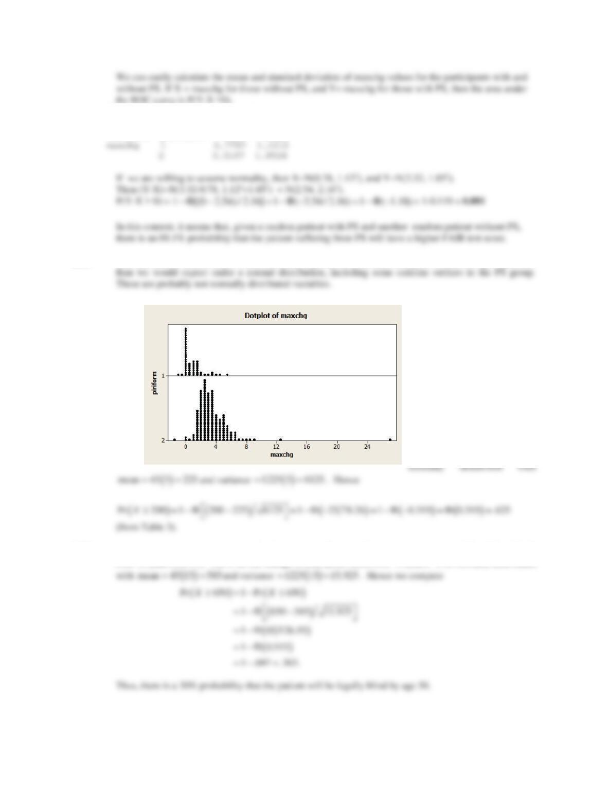
5.84 The ROC curve is shown below, where sensitivity and specificity are evaluated for every value of
‘maxchg’.
84 CHAPTER 5/CONTINUOUS PROBABILITY DISTRIBUTIONS
Descriptive Statistics: maxchg
Variable piriform Mean StDev
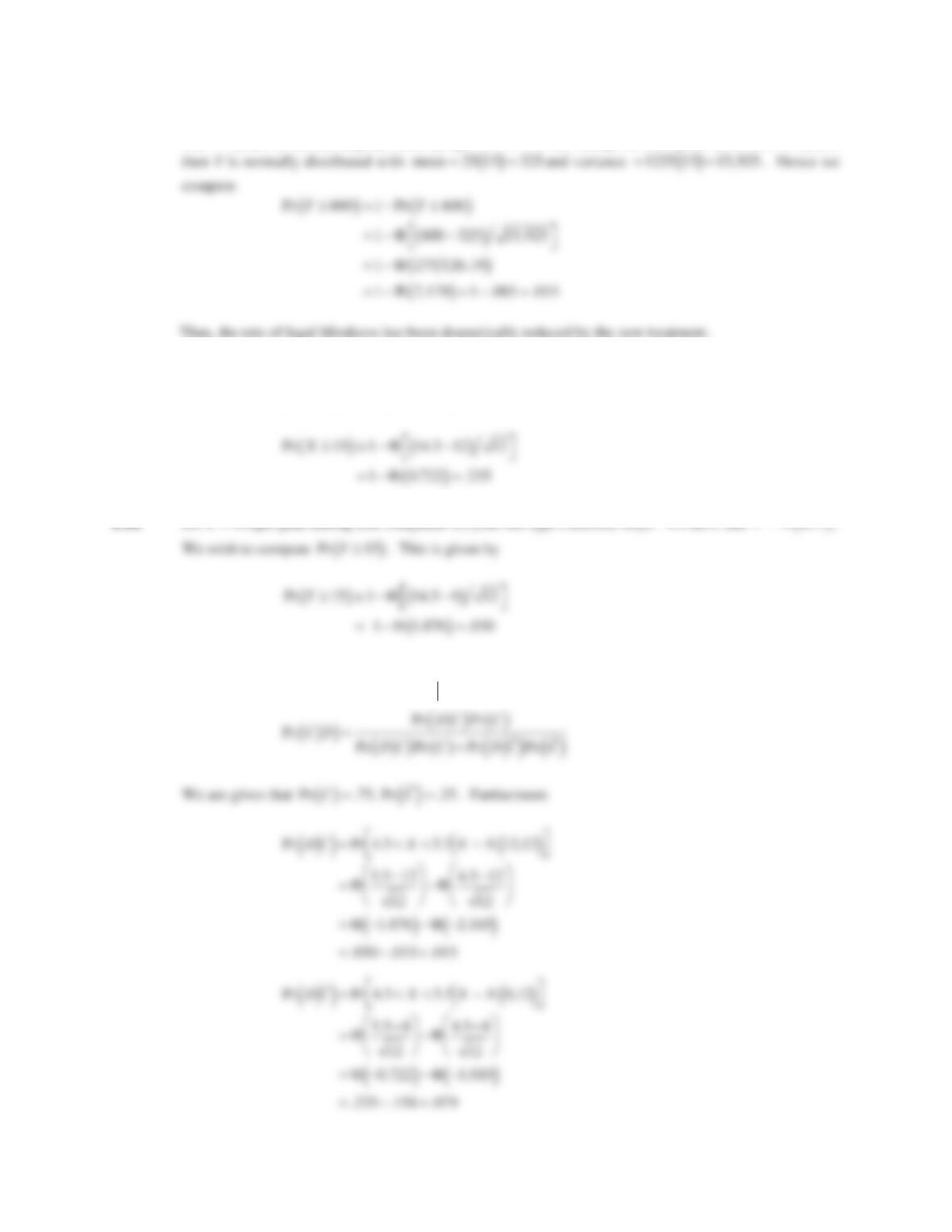
5.85 The distribution of FAIR test scores within each group is unimodal, but appears to have longer right tails
5.86 Let X = change over 5 years. X is
5.87 In order for the patient to be legally blind by age 50, he will have to decline by 900 250 650t db
over 13 years (50-37). Let X be the change in total point score over 13 years. X is normally distributed
CHAPTER 5/CONTINUOUS PROBABILITY DISTRIBUTIONS 85
5.88 After the treatment the total point score for this patient will be 850 db. He must decline by 600tdb
over 13 years to become legally blind by age 50. If Y is the change in total point score over 13 years,
5.89 Let X = weight gain among compliant 12-year-old-type I diabetic boys. We have that
12,12XN.
We wish to compute
Pr 15Xt. This is given by
5.90 Let Y = weight gain among non-compliant 12-year-old-type I diabetic boys. We have that
8,12YN.
5.91 Let C be the random variable representing compliance. Let D be the random variable representing a 5 lb.
weight gain. We wish to compute
Pr CD . From Bayes’ Theorem, we have
86 CHAPTER 5/CONTINUOUS PROBABILITY DISTRIBUTIONS
Therefore, upon substitution
5.93 If the level of pollution has no association with the onset of heart attack, then 12p , where p =
probability that the pollution level on the index date is greater than the pollution level on the control date
5.95 Let X be serum lutein for placebo subjects. We have
CHAPTER 5/CONTINUOUS PROBABILITY DISTRIBUTIONS 87
5.97 Let T be the event that serum lutein is in the therapeutic range (i.e., 10 mg/dlt). We use the total
probability rule. Let M = macular degeneration. We have
5.98 We first compute the probability of macular degeneration for placebo-treated subjects. We have
5.100 Let X = number of IVF infants with at least one birth defect. X is binomially distributed with 837n and
5.101 In this case, if X = number of IVF infants with chromosomal birth defects, then X is binomially
88 CHAPTER 5/CONTINUOUS PROBABILITY DISTRIBUTIONS
5.103 Using Excel, P(X5) = 1-BINOMDIST(4,20,0.065,1) = 0.008. This suggests that it is highly unlikely
5.107 From 5.103, we know that the 40th percentile of a standard normal distribution is -0.25, and so the 60th
percentile is 0.25. Now,
5.109 In the study, the probability of a low birthweight delivery is 5.7%, so if 20 women are chosen randomly
5.112
CHAPTER 5/CONTINUOUS PROBABILITY DISTRIBUTIONS 89
P(smokes) = P(smokes | Category j)uP(Category j)
j A
E
¦
P(low birthweight | smokes) = P(low birthweight & smokes)/P(smokes)
5.113 If we assume that the number of breast cancer cases X comes from a Poisson distribution with mean =
5.114 The cumulative incidence for breast cancer between the ages of 40-64 will be the sum of the annual
incidence rate at each age. From Table 5.7, we see five different incidence rates, each of which are
5.115
10,000,000u2.35
§
¨
·
¸ 10
7
/10
2
u(2.35) 2.35u10
5
5.116 Prevalence tells how many total cases of cancer exist in a population. Incidence tells how many new
cases of cancer appear in a population.
90 CHAPTER 5/CONTINUOUS PROBABILITY DISTRIBUTIONS
5.120 Relative risk = P(AMD|CC genotype) / P(AMD|TT genotype) = [121/(121+278)] / [41/(41+380)]
5.121 In the 1185 subjects without AMD, there are 2 x 1185 = 2370 alleles in total.
5.122 From 5.118, we expect 1185*(0.496) = 587.76 individuals without AMD to show the TC genotype.
5.123
V
w
2
V
A
2
/n
V
2
/nk 42.9 / 2 12.8 / 4 24.65
5.124 We want
(| | 5) 0.05
(| | / 5 / ) 0.05
ww
P
X
PX
P
PV V
!
!
CHAPTER 5/CONTINUOUS PROBABILITY DISTRIBUTIONS 91
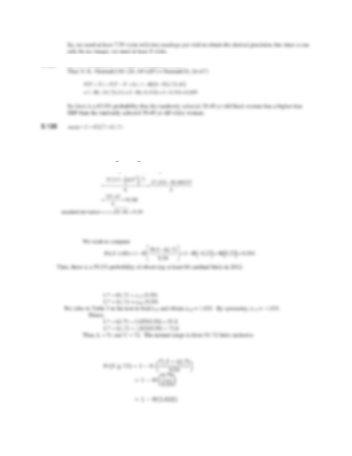
5.125 Let X~Normal(120, 142), and Y~Normal(130, 202)
5.127
variance s
2
1
6x
i
2
i 1
7
¦
1
7x
i
i 1
7
¦
§
©
¨
¨
·
¹
¸
¸
2
ª
«
«
«
º
»
»
»
5.128 Let X = number of cardinal birds observed in 2012.
5.129 We know that the 15th and 85th percentiles (L*, U*) are given by
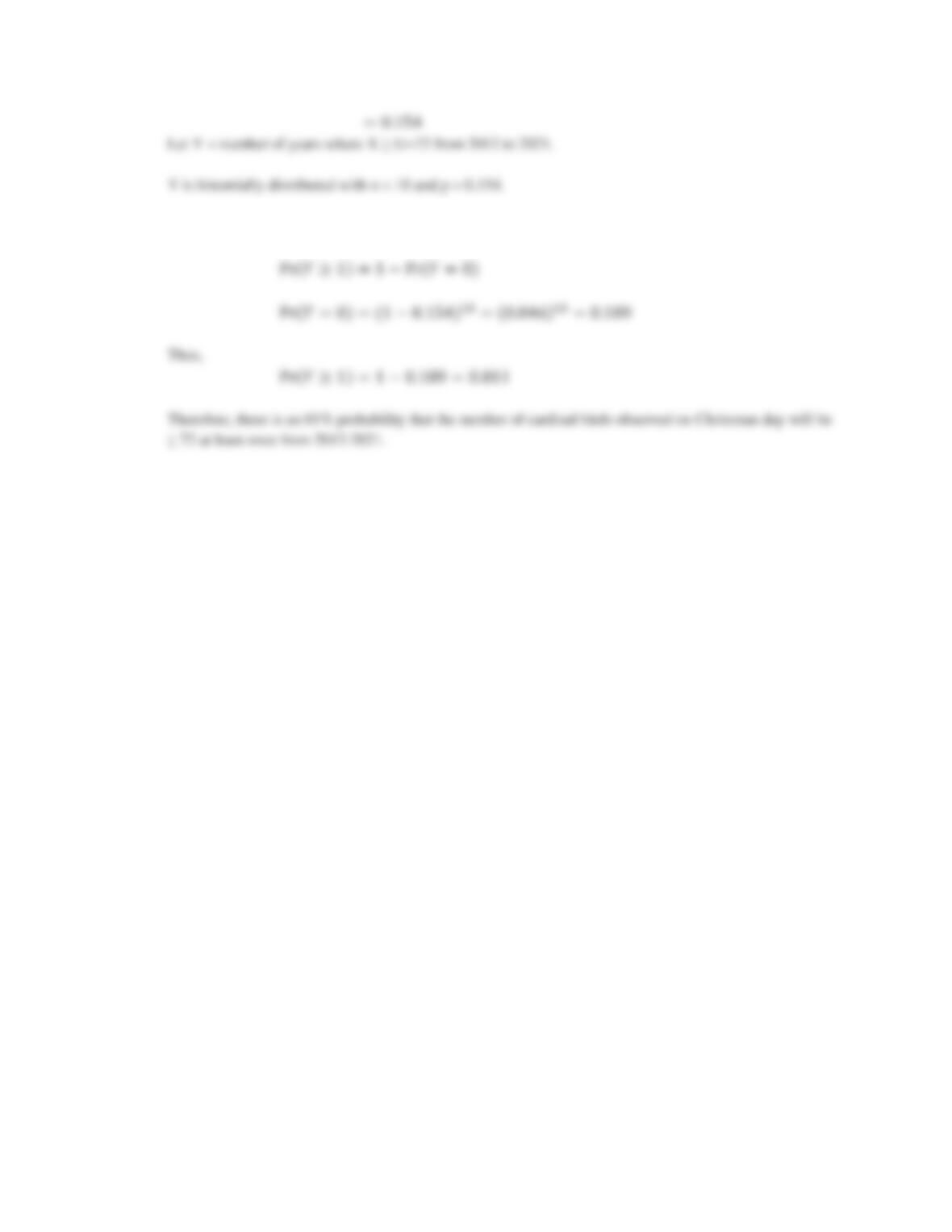
5.130We know that
92 CHAPTER 5/CONTINUOUS PROBABILITY DISTRIBUTIONS
We wish to compute
ሺܻͳ