65
CONTINUOUS
PROBABILITY
DISTRIBUTIONS
5.6 If X represents total carbohydrate intake in 12–14-year-old males, then we compute
5.7 We compute
5.8 Let Y represent carbohydrate level in 1214-year-old boys below the poverty level. We wish to compute
5.9 We compute
66 CHAPTER 5/CONTINUOUS PROBABILITY DISTRIBUTIONS
5.10Let D = delta. We have:
Pr(Dt2) 1) 20.189
2.428
§
¨
·
¸
5.11 We denote the 90th and 10th percentile of D by D90 and D10, respectively. We have:
D
0.189 z
(2.428)
5.12 We have that
X~N12.8, 5.1
2
. We wish to compute . We have
5.13 Here,
X~N9.3, 3.2
2
. We wish to compute . We have that
5.14 Let serum cholesterol. Compute
Pr X !
20
Pr X !
20
X
CHAPTER 5/CONTINUOUS PROBABILITY DISTRIBUTIONS 67
5.15 We want
5.16 We want
¹
§
·
§
·
5.17 We have
p
1
Pr 1 to 14-year-old is hypertensive
Pr systolic bp !115
5.18 Similarly, we let
p2 Pr systolic bp !140
5.19 A family is hypertensive if at least one adult and at least one child is hypertensive.
68 CHAPTER 5/CONTINUOUS PROBABILITY DISTRIBUTIONS
5.20 The number of hypertensive families in the apartment building (X) follows a binomial distribution with
parameters 1000n and .0058p . Thus, we have
5.21 This is given by
5.22 This is given by
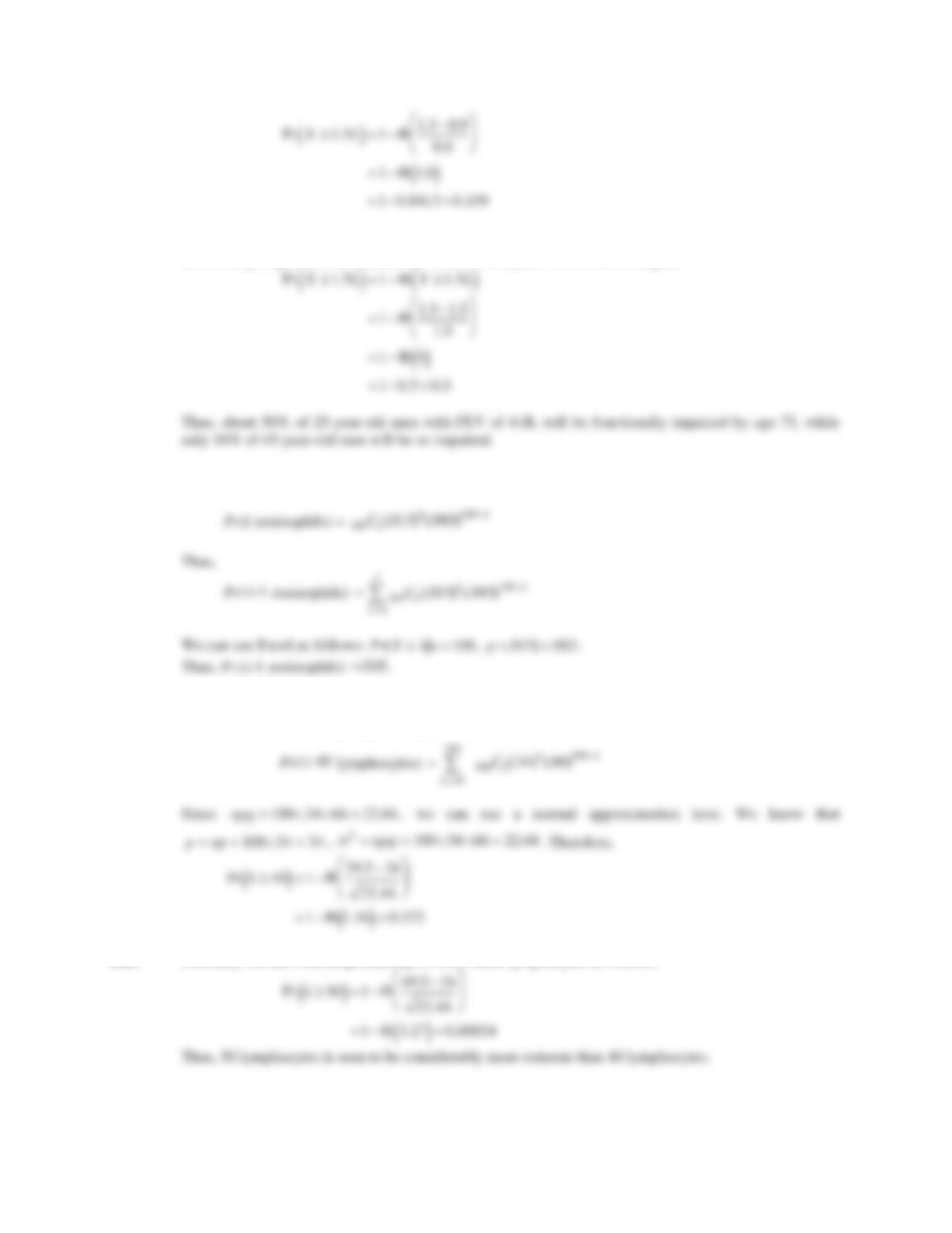
5.23 The mean decline in FEV for such a 75-year-old man will be . The standard deviation of
003 30 09..
L
CHAPTER 5/CONTINUOUS PROBABILITY DISTRIBUTIONS 69
5.24 Here the mean decline in FEV will be with . The man will be
functionally impaired if he declines by 1.5L over 50 years. We wish to compute
5.25 We have Pr eosinophils) Pr eosinophils), where
5.26 We have that
Pr(k lymphocytes)
5.27 Similarly, we can find the probability of 50 or more lymphocytes as follows:
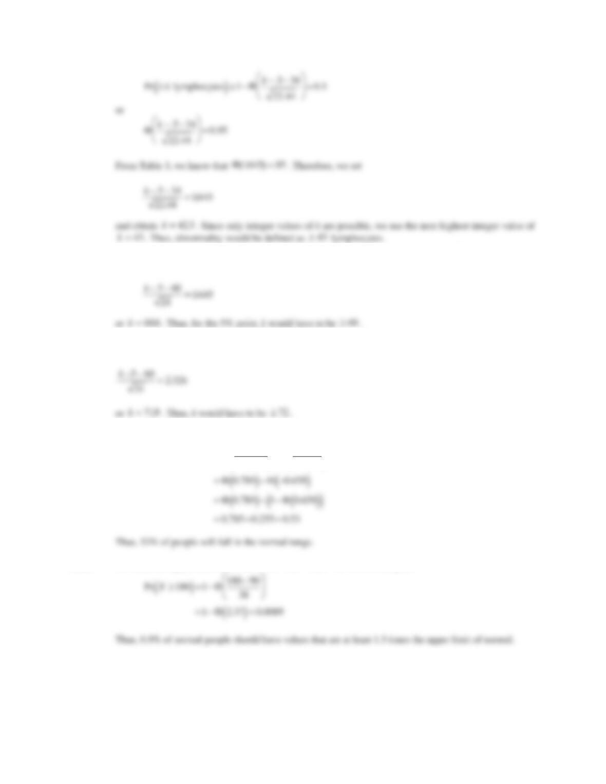
5.28 One approach to this problem is to find a k such that Pr lymphocytes) .
If we use a normal approximation, then we have
00350 15..
Lsd L
002 50 10..
(t5 1(d4
100
100
34 66Ck
kk
..
(tk#.05
70 CHAPTER 5/CONTINUOUS PROBABILITY DISTRIBUTIONS
5.29 We can use the same approach with neutrophils. Specifically, we have , .
We find k such that
5.30 Since , we need to find a k that satisfies the equation
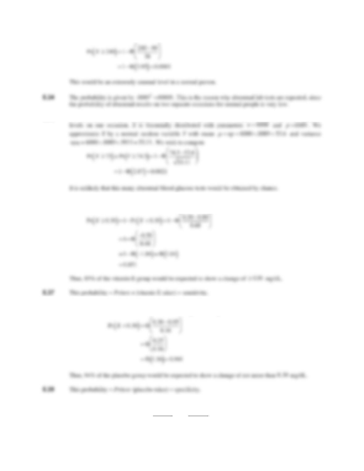
5.31 If the random variable X represents blood glucose, then we wish to compute
Pr 65 dXd120
) 120 90
38
§
©
¨
·
¹
¸) 6590
38
§
©
¨
·
¹
¸
5.32 1.5 times the upper limit of normal . We wish to compute
5.33 Since , we evaluate
P
60
V
2100 6 4 24 uu ..
)2 326 99..
u 1 5 120 180.
2 120 240u
CHAPTER 5/CONTINUOUS PROBABILITY DISTRIBUTIONS 71
5.35 Let the random variable X represent the number of patients in the study with abnormal blood-glucose
5.36 We wish to compute where
X~N0.8, 0.48
2
. We have
5.38 We wish to compute where
X~N0.05, 0.16
2
. We have
5.40 If our threshold , then
sensitivity
1) ‘0.80
0.48
§
©
¨
·
¹
¸ ) 0.80 ’
0.48
§
©
¨
·
¹
¸
Pr X t
030.
Pr X
030.
‘
72 CHAPTER 5/CONTINUOUS PROBABILITY DISTRIBUTIONS
©
¹
Thus, the compliance would be 88% in each group using this measure of compliance.
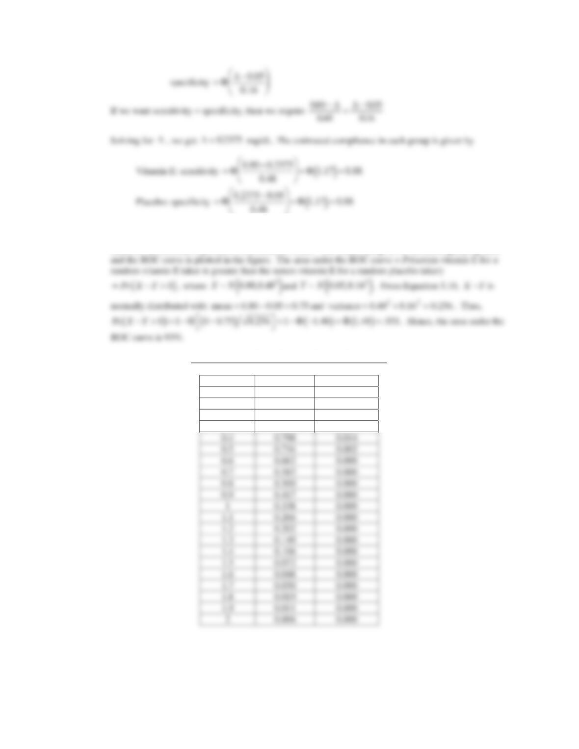
5.41 We will choose
0,0.10,…, 2.0‘ and compute the sensitivity and (1 – specificity) for each cutpoint
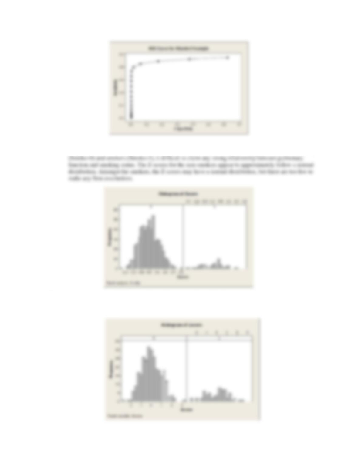
based on the formula in problem 5.50 based on Excel. The results are given in the accompanying table
Sensitivity vs. 1-Specificity for Vitamin E Example
Cutpoint Sensitivity 1-Specificity
0 0.952 0.623
0.1 0.928 0.377
0.2 0.894 0.174
0.3 0.851 0.059
CHAPTER 5/CONTINUOUS PROBABILITY DISTRIBUTIONS 73
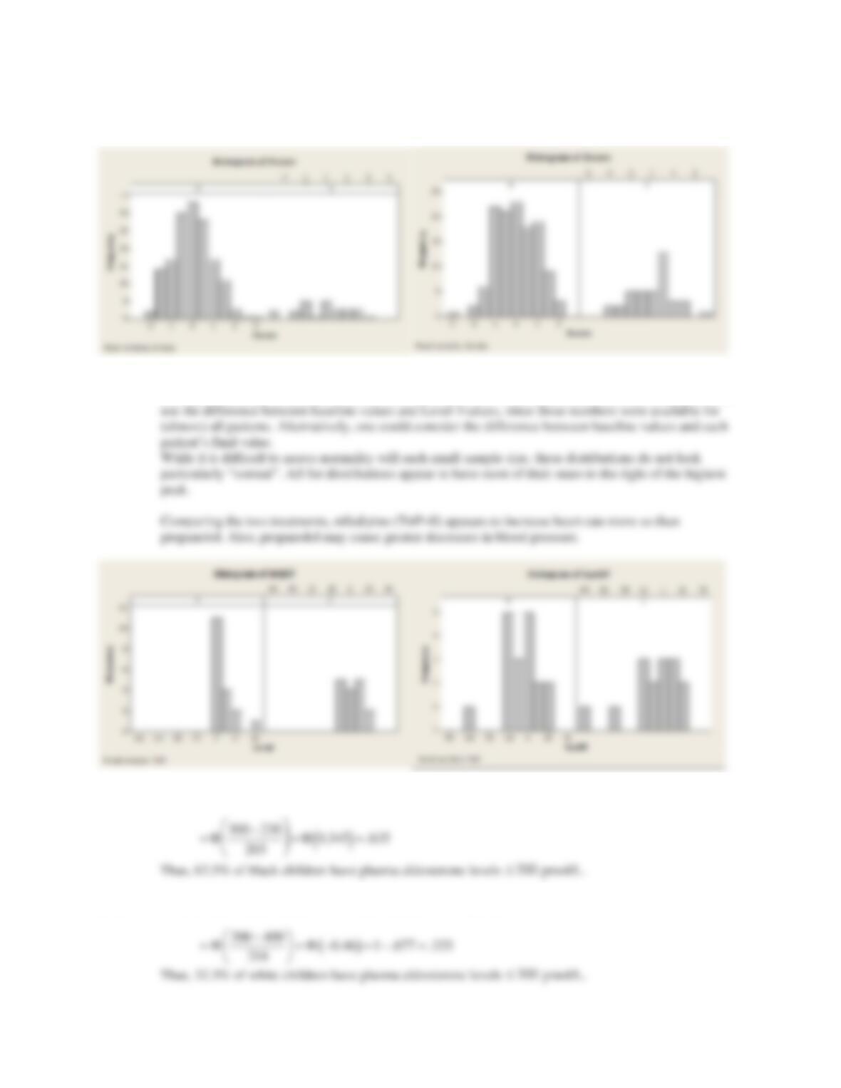
5.42 After creating age-sex IDs for each group, we note that 4 of the 34 groups have only one child. We will
assign a Z-score of 0 for each of these 4 children. When we plot histograms of Z-scores for non-smokers
5.43 If we only look at children age 10 or older, we reach roughly the same conclusions. We note that the
peak of the distribution for non-smokers appears to be slightly below 0, while the peak for the smokers
appears to be slightly above 0.
74 CHAPTER 5/CONTINUOUS PROBABILITY DISTRIBUTIONS
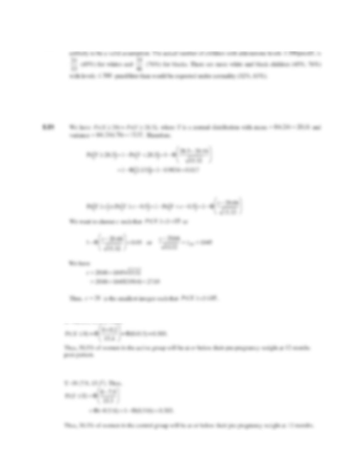
5.44 Whether we consider boys age 10 or older (left panel) or girls age 10 or older (right panel), we still
cannot determine any relationship between FEV level and smoking status.
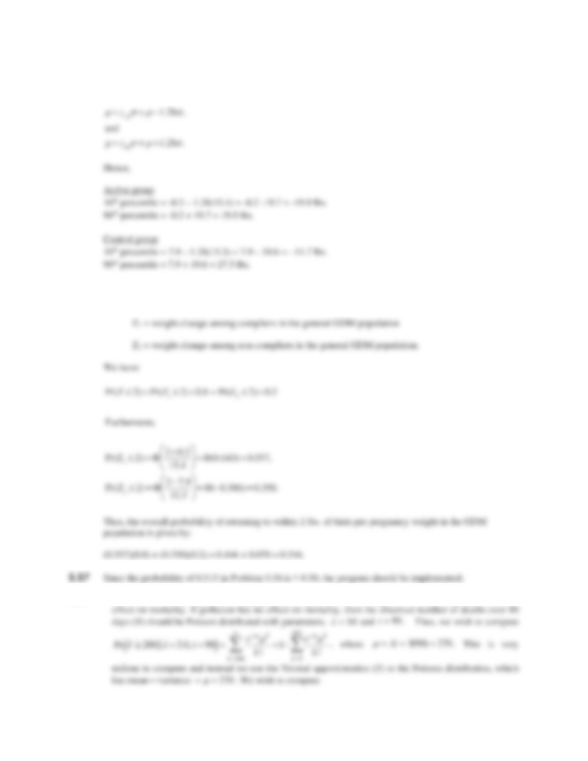
5.45-46 For this analysis, we need to create new variables representing change in heart rate (HrtDif), change in
blood pressure (SysDif), and a treatment indicator (here TrtP for propanolol). For HrtDif and SysDif, we
5.47 If normality is assumed, the % of black children pmol/L
5.48 If normality is assumed, the % of white children pmol/L
d300
d300
CHAPTER 5/CONTINUOUS PROBABILITY DISTRIBUTIONS 75
5.49 The distribution of aldosterone in both blacks and whites appears to be very skewed, and normality is
5.50 The probability is given by
84
29
§
©
¨
¨
¨
·
¹
¸
¸
¸0.24
29
0.76
55
. Using Excel, this is given by .009.
5.52 Suppose the critical value c. We have the relationship
5.53Let X = 12 month weight – pre-pregnancy weight for women in the active group. We know that
5.54Let Y = 12 month weight – pre-pregnancy weight for women in the control group. We know that
76 CHAPTER 5/CONTINUOUS PROBABILITY DISTRIBUTIONS
5.55The 10th and 90th percentiles are given by:
5.56
Let Z = weight change in the general GDM population
5.58 We observe 288 deaths over 90 high pollution days, whereas we expect 270 deaths if pollution has no
CHAPTER 5/CONTINUOUS PROBABILITY DISTRIBUTIONS 77
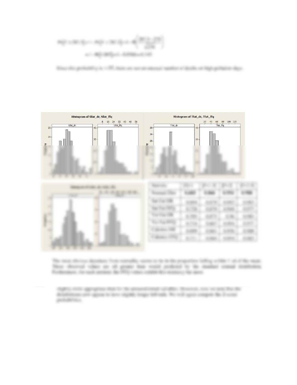
5.59 Histograms for each of the variables are shown below, with DR values on the left panel and FFQ values
on the right panel of each plot. Each of the distributions is unimodal, but they all appear to have longer
right tails than left tails. Thus, a normal distribution may not be appropriate; we can convert each of the 6
columns under investigation into Z-scores and count the number that fall within “X” standard deviations
of the mean.
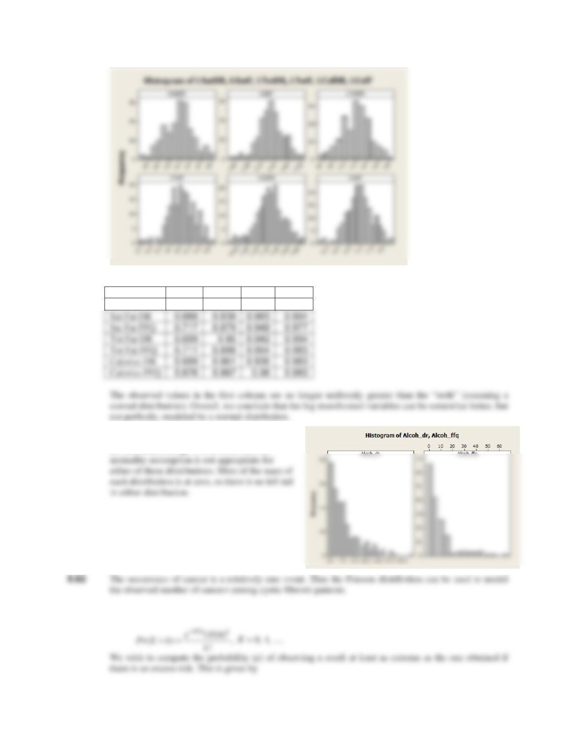
5.60 After taking the ln-transformation of each variable, it appears that the normality assumption may be
78 CHAPTER 5/CONTINUOUS PROBABILITY DISTRIBUTIONS
Log-transformed variables
Statistic |Z|<1 |Z<1.5| |Z<2| |Z<2.5|
Normal Dist 0.683 0.866 0.954 0.988
5.61 The DR and FFQ values for alcohol consumption
are unimodal, though it is obvious that the
5.63 The probability of observing kcancers if there is no excess risk among cystic fibrosis patients is given by