Chapter 5
Cost Estimation
Learning Objectives
1. Understand the reasons for estimating fixed and variable costs.
2. Estimate costs using engineering estimates.
4. Estimate costs using statistical analysis.
6. Identify potential problems with regression data.
8. Evaluate the advantages and disadvantages of alternative cost estimation methods.
10. (Appendix B) Understand the mathematical relationship describing the learning phenomenon.
Chapter Overview
I. WHY ESTIMATE COSTS?
II. BASIC COST BEHAVIOR PATTERNS
III. WHAT METHODS ARE USED TO ESTIMATE COST BEHAVIOR?
• Engineering Method
• Account Analysis Method
• Statistical Cost Estimation
o Relevant Range of Activity
o Scattergraphs and High-Low Estimates
o Number of Observations
• Multiple Regression
• Practical Implementation Problems
o Effect of Nonlinear Relations
o Effect of Outliers
o Effect of Spurious Relations
IV. LEARNING PHENOMENON
• Applications
o Decision Making
o Performance Evaluation
V. HOW IS AN ESTIMATION METHOD CHOSEN?
• Data Problems
• Effect of Different Methods on Cost Estimates
Chapter Outline
LO 5-1 Understand the reasons for estimating fixed and variable costs.
WHY ESTIMATE COSTS?
• When managers make decisions, they need to compare the costs and benefits among
alternative actions.
BASIC COST BEHAVIOR PATTERNS
• The most important characteristic of costs for decision making is how they behave.
o Key terms for describing cost behavior:
▪ Variable costs change proportionately with activity levels. (See Business Application
box “Understanding Fixed and Variable Costs for Online Sales.”)
▪ Fixed costs do not vary with activity levels.
WHAT METHODS ARE USED TO ESTIMATE COST BEHAVIOR?
• Three general methods are used to estimate the relation between cost behavior and activity
levels.
o In practice, operating managers frequently apply their own best judgment as a final step
in the estimation process.
LO 5-2 Estimate costs using engineering estimates.
• Engineering Method
o An engineering estimate is a cost estimate based on measurement and pricing of the
work involved in a task.
▪ A detailed step-by-step analysis is performed of what needs to be done; that is, the
activities that must be conducted. The times or costs are then estimated for each
activity.
o Advantages of engineering estimates:
▪ It can detail each step required to perform an operation permitting comparison with
similar operations in order to review productivity and to identify strengths and
weaknesses.
▪ It does not require data from prior activities in the organization; hence, it can be used
to estimate costs for totally new activities.
LO 5-3 Estimate costs using account analysis.
• Account Analysis Method
o Account analysis is a cost estimation method that calls for a review of each account
making up the total cost being analyzed.
▪ Each cost is identified as fixed or variable, depending on the relation between the cost
and some activity.
▪ The key step in account analysis is the identification of the relation between the
activity and the resulting cost; the identification depends on the accountant’s
judgment and experience.
o Exhibit 5.1 shows an example of cost estimation using account analysis; in this example:
o Account analysis helps determine the fixed cost (F) and the variable cost per unit (V) in
the cost equation: TC = F + VX.
▪ An estimate of the total cost (TC) in the future can be made for other activity levels
(X) as long as they are within the relevant range of the operations.
See Demonstration Problem 1
LO 5-4 Estimate costs using statistical analysis.
• Statistical Cost Estimation
o When random and unusual events are present, statistical analysis can use data from the
past several periods of operations or several locations as the basis for estimating cost
relations.
o Relevant Range of Activity
▪ When using statistical approaches to cost estimation, we need to ensure that the
activity levels of the past are relevant for the activity levels estimated. Extrapolations
beyond the upper and lower bounds of past observations are highly subjective.
o Scattergraphs and High-Low Estimates
▪ A scattergraph is a graph that plots costs against activity levels.
• This visual representation of the data provides a quick indication of the fixed-
variable relation of costs and activities.
• It also indicates if the relation seems to change at certain activity levels.
▪ Exhibit 5.2 shows the data and a scattergraph for a representative center.
o Number of Observations
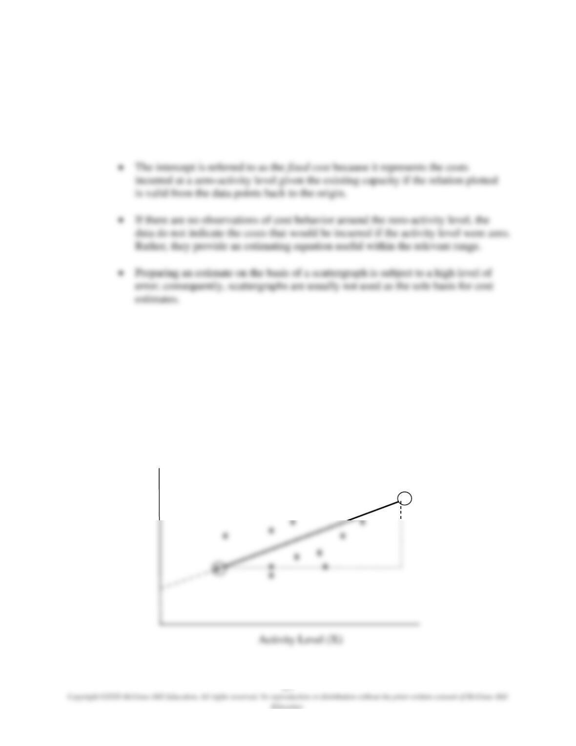
▪ A line can be visually fitted (by way of “eyeball judgment”) to the data points as
closely as possible and extended to the vertical axis on the scattergraph.
• The slope of the line represents the estimated variable cost per unit; the slope is
referred to as the variable cost per unit because it represents the change in costs
that occurs as a result of changes in activity.
o High-Low Cost Estimation
▪ High-low cost estimation is the method that estimates costs based on two cost
observations, usually at the highest and lowest activity levels.
▪ The following is a generic representation of a scattergraph and a fitted line based on
the highest and lowest activity levels. The coordinates for the lowest point and the
highest point are circled.
Total Cost (Y=TC)
x
x
x
• The slope of the total cost line, which estimates the increase in variable costs
associated with an increase of one unit of activity, can be estimated using the
following equation:
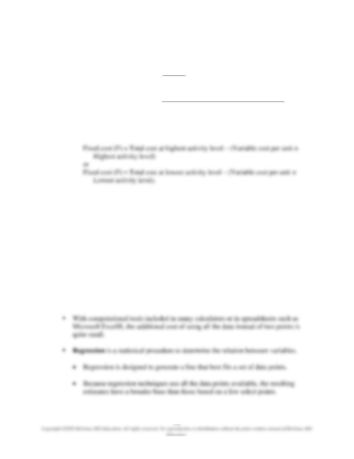
Variable cost per unit (V) =
y2 – y1
x2 – x1
=
Cost at highest activity – Cost at lowest activity
Highest activity – Lowest activity
• Next, the intercept is estimated by taking the total cost at either activity level and
subtracting the estimated variable cost:
• An estimate of the costs for any given activity level can then be computed using
the cost equation: TC = F + VX.
▪ The high-low method is easy to apply, but must be used carefully to ensure that the
two points chosen to prepare the estimates represent cost and activity relations over
the range of activity for which the prediction will be made.
• When the scattergraph indicates that the highest and/or lowest points represent
unusual circumstances, other more representative highest and/or lowest point
should be chosen instead.
See Demonstration Problem 2
o Statistical Cost Estimation Using Regression Analysis
LO 5-5 Interpret the results of regression output.
o Obtaining Regression Estimates
▪ The most important step in obtaining regression estimates for cost estimation is to
establish the existence of a logical relation between activities and the cost to be
estimated.
▪ Entering numbers that have no logical relation can result in misleading estimates; the
activities (i.e., independent variables) must be logically related to costs to be
estimated (i.e., dependent variables).
▪ A simple regression uses just a single predictor.
• The intercept term from the output of a regression program is an estimate of fixed
cost; the intercept at zero activity it is usually outside the relevant range of
observations.
• The coefficient of the X term is an estimate of the variable cost per unit of activity;
this is the slope of the cost line. The coefficients are often labeled as b or given
the variable name on the program output.
o Correlation Coefficients
▪ In addition to the cost-estimating equation, the regression program provides other
useful statistics.
• Correlation coefficient (R, or Multiple R) is a measure of the linear relation
between two or more variables, such as cost and some measure of activity.
• The square of R (or R2) is called the coefficient of determination; it is the square
of the correlation coefficient, interpreted as the proportion of the variation in the
dependent variable explained by the independent variable(s).
▪ Example: The regression results in Exhibit 5.3 where the linear relation between
overhead cost and repair-hours used is estimated are as follows:
Correlation coefficient (R) … .856
R2 …………………………… .733
▪ The most commonly used regression technique is called ordinary least squares
regression (OLS).
• With this technique, the regression line is computed so that the sum of the squares
of the vertical distances from each point to the regression line is minimized.
o Confidence in the Coefficients
▪ In many cases, it can be desirable to determine whether the estimated coefficient on
the independent variable is significantly different from zero. For example, when
determining fixed and variable costs, if the estimated coefficient is significantly
different from zero, we can conclude that the cost is not totally fixed.
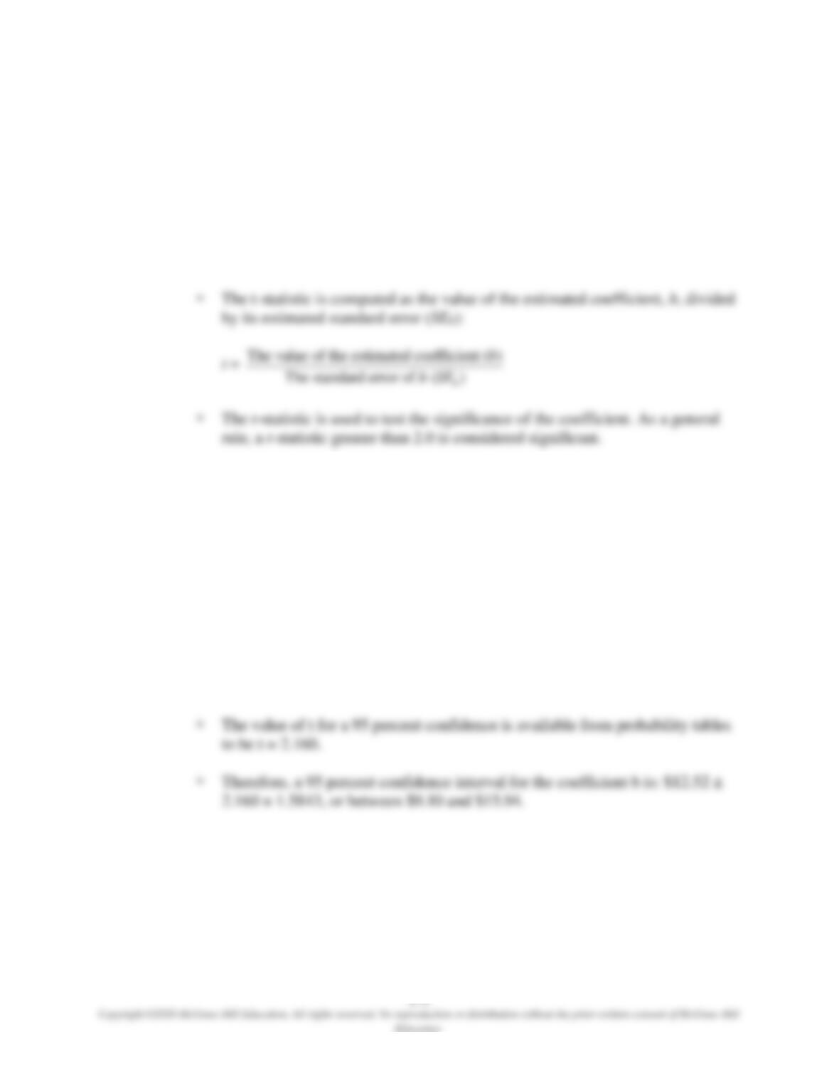
• The t-statistic is used to test the significance of the coefficient; the t-statistic, t, is
the value of the estimated coefficient, b, divided by its standard error.
• The significance level of the t statistic is called the p-value. A very small p-value
(close to zero) means that the probability that the true value of the coefficient is
zero, given the data, is virtually zero.
• To construct a 95% confidence interval around b, we add or subtract to b the
appropriate t-value for the 95% confidence interval times the standard error of b
as follows: b ± t × SEb. That is, with a 95% probability, the variable cost
coefficient should be between (b – t × SEb) and (b + t × SEb).
• Example: From the regression results in Exhibit 5.3, where the linear relation
between overhead cost and repair-hours used is estimated, b = $12.52 and SEb =
1.5843.
See Demonstration Problem 3
• Multiple Regression
o See Business Application box “Using Statistical Analysis to Improve Profitability.”
o Management might wish to see whether a better estimate can be obtained using additional
predictor variables.
o The adjusted R-squared (R2) is the correlation coefficient squared and adjusted for the
number of independent variables used to make the estimate.
▪ This adjustment to R2 recognizes that as the number of independent variables
increases, R2 (unadjusted) increases.
• Statisticians believe that adjusted R2 is a better measure of the association
between X and Y than the unadjusted R2 value when more than one X predictor is
used.
• The t-statistic for each of the coefficients can also be tested for significance. That
is, a particular factor can be tested to see if it is indeed a cost driver.
▪ The additional data requirements for multiple regression models may limit their
usefulness in many applications.
LO 5-6 Identify potential problems with regression data.
• Practical Implementation Problems
o Some of the more common problems with using regression estimates include:
▪ Attempting to fit a linear equation to nonlinear data,
o Effect of Nonlinear Relations
▪ The effect of attempting to fit a linear model to nonlinear data is likely to occur when
the firm is operating near its capacity limits.
▪ One way to overcome the problem is to define a relevant range of activity and use the
range for one set of cost-estimating regression equations.
• A different equation could be derived for the levels between 81 and 100 percent
capacity.
▪ Another approach is to model the nonlinearity explicitly by including the squared
value of an independent variable as well as the variable itself.
• This approach does not provide a constant unit variable cost estimate; the estimate
is different at each level of activity.
o Effect of Outliers
▪ Because regression minimizes the sum of the squared deviations from the regression
line, observations that lie a significant distance away from the line could have an
overwhelming effect on the regression estimates.
▪ Exhibit 5.6 shows a case in which most of the data points lie close to a straight line,
but because of the effect of one significant outlier, the computed regression line is a
substantial distance from most of the points.
o Effect of Spurious Relations
▪ Spurious relations may result from including many variables in the regression in the
hope of finding relations among the variables.
o Effect of Using Data that Do Not Fit the Assumptions of Regression Analysis
▪ Two important assumptions that are often not satisfied in estimating costs are that:
• The process for which costs are being estimated remains constant over time, and
• The errors in estimating the costs are independent of the cost drivers.
o Regression Must Be Used with Caution
▪ A regression estimate is only an estimate; users should:
LO 5-7 Incorporate the effects of learning when estimating costs.
LEARNING PHENOMENON
• Learning affects labor costs. The more experience that workers have in performing a task, the
less time they spend on it.
o The learning phenomenon refers to the systematic relationship between the amount of
experience in performing a task and the time required to perform it.

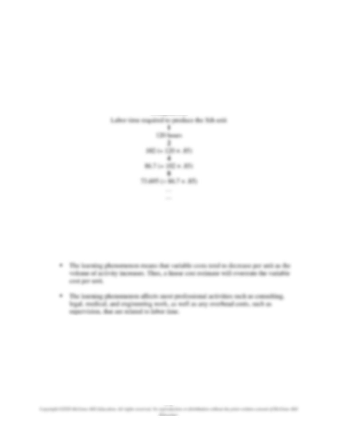
o Example: Using the incremental unit-time learning model with an 85 percent learning
rate for workers, whenever the output units are doubled (say from the first unit to the
second unit or from the second unit to the fourth unit, and so on), the time it takes to
produce the new output volume will be 85 percent of what it took to produce half of it
previously.
▪ That is:
Unit
▪ Appendix B presents the mathematical formula for deriving the learning curve and
extends this example.
• Applications
o Decision Making
o Performance Evaluation
▪ Failing to recognize learning effects can have some unexpected consequences in
decision making and performance evaluation, among others.