Problem 5A-7 (45 minutes)
1.
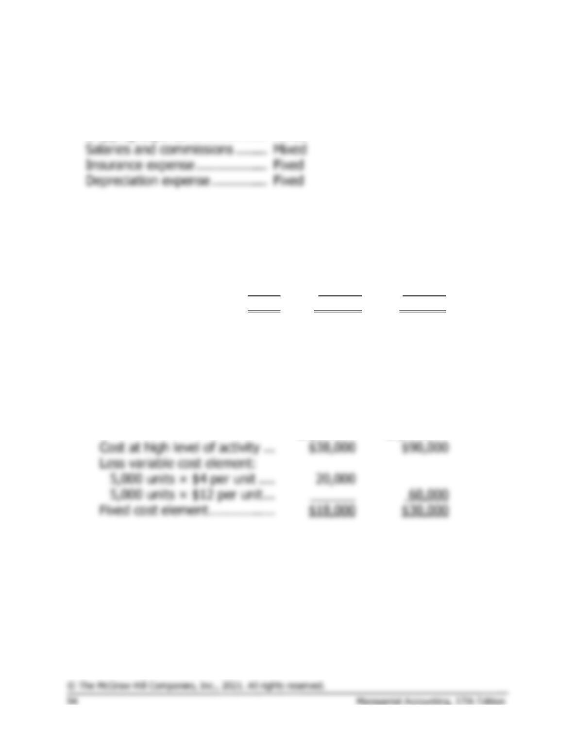
Cost of goods sold ……………….
Variable
Advertising expense …………….
Fixed
Shipping expense ………………..
Mixed
Salaries and commissions ……..
Mixed
2. Analysis of the mixed expenses:
Units
Shipping
Expense
Salaries and
Commissions
Expense
High level of activity …..
5,000
$38,000
$90,000
Low level of activity ……
4,000
34,000
78,000
Change ……………………
1,000
$ 4,000
$12,000
Variable cost element:
Fixed cost element:
Shipping
Expense
Salaries and
Commissions
Expense
Cost at high level of activity …
Fixed cost element ……………..
Problem 5A-7 (continued)
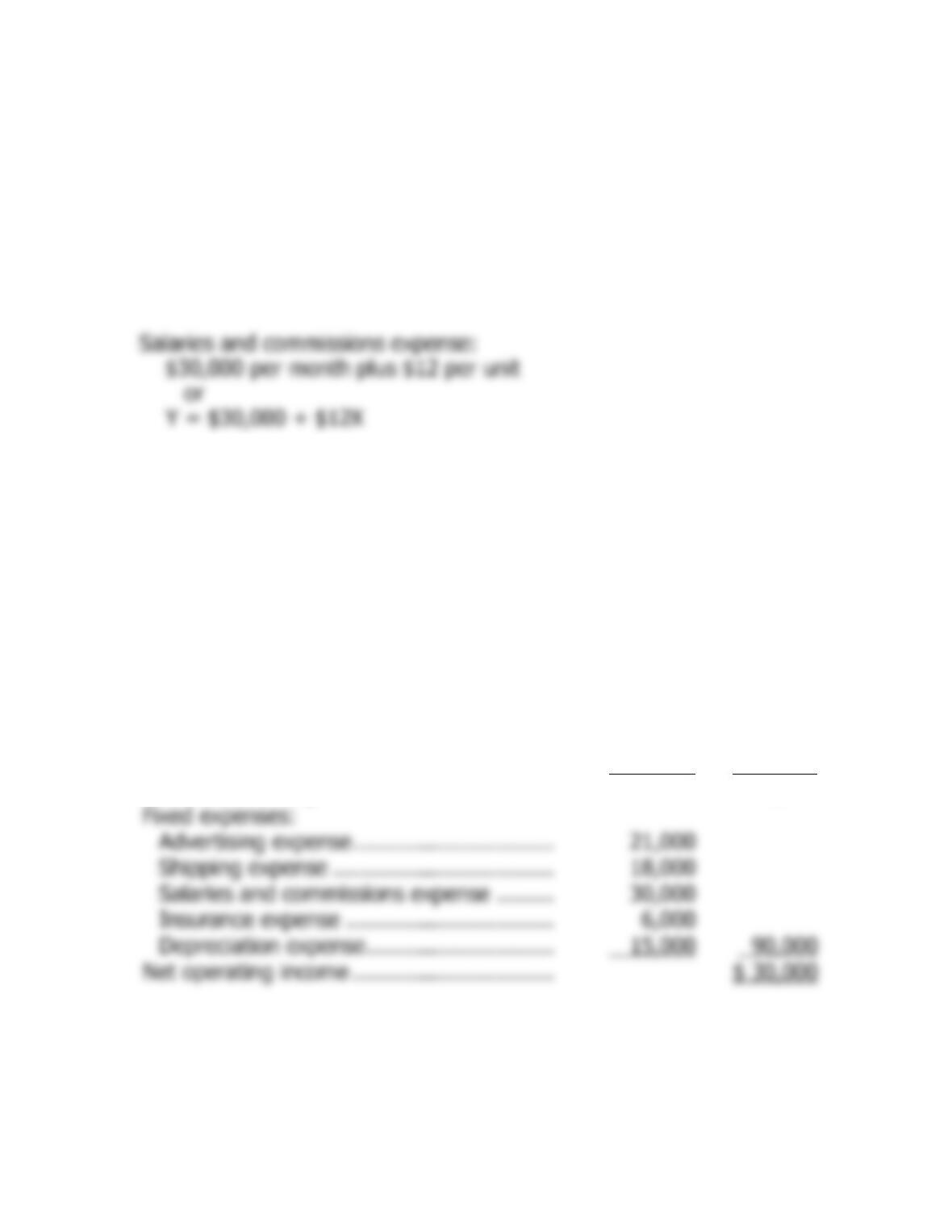
The cost formulas are:
Shipping expense:
$18,000 per month plus $4 per unit
or
Y = $18,000 + $4X
3.
Morrisey & Brown, Ltd.
Income Statement
For the Month Ended September 30
Sales (5,000 units × $100 per unit) ………..
$500,000
Variable expenses:
Cost of goods sold
(5,000 units × $60 per unit) …………….
$300,000
Shipping expense
(5,000 units × $4 per unit) ………………
20,000
Salaries and commissions expense
(5,000 units × $12 per unit) …………….
60,000
380,000
Contribution margin …………………………...
120,000
Fixed expenses:
21,000
15,000
Net operating income ………………………….
$ 30,000
Problem 5A-8 (20 minutes)
1. Maintenance cost at the 90,000 machine-hour level of activity can be
isolated as follows:
Level of Activity
60,000 MHs
90,000 MHs
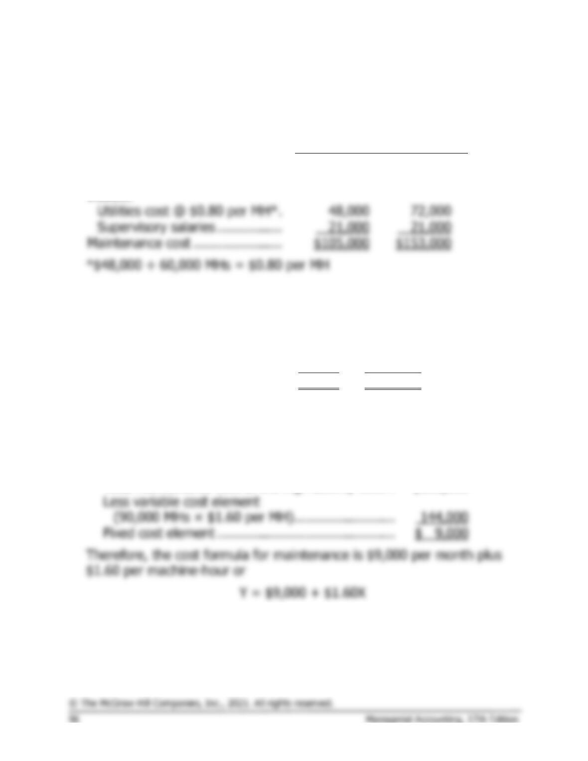
Total factory overhead cost ……..
$174,000
$246,000
Deduct:
Maintenance cost ………………….
2. High-low analysis of maintenance cost:
Machine-
Hours
Maintenance
Cost
High activity level ………………..
90,000
$153,000
Low activity level …………………
60,000
105,000
Change ……………………………..
30,000
$ 48,000
Variable rate:
Change in cost/Change in activity = $48,000/30,000 MHs = $1.60
per MH
Total fixed cost:
Total maintenance cost at the high activity level ..
$153,000
Fixed cost element ……………………………………..
Problem 5A-8 (continued)
3.
Variable Cost per
Machine-Hour
Fixed Cost
Utilities cost ………………..
$0.80
Supervisory salaries cost ..
$21,000
Maintenance cost …………
1.60
9,000
Total overhead cost ………
$2.40
$30,000
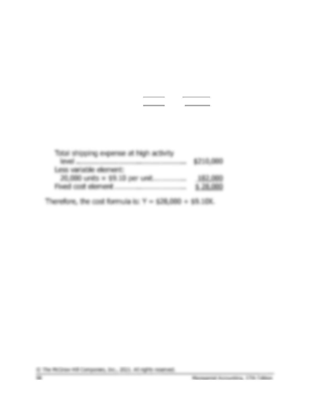
Thus, the cost formula would be: Y = $30,000 + $2.40X.
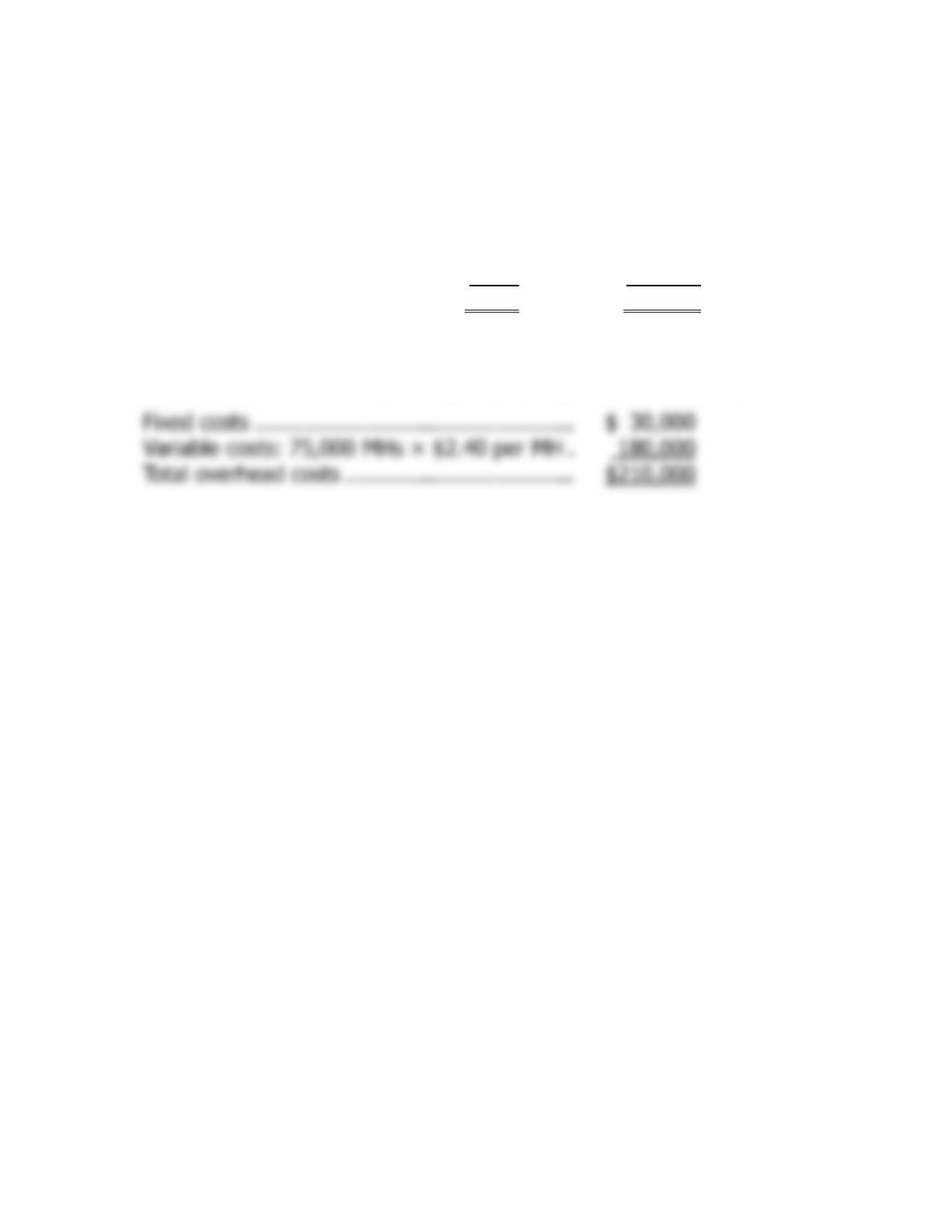
4. Total overhead cost at an activity level of 75,000 machine-hours:
Fixed costs ………………………………………….
Variable costs: 75,000 MHs × $2.40 per MH .
Total overhead costs ……………………………..
Problem 5A-9 (30 minutes)
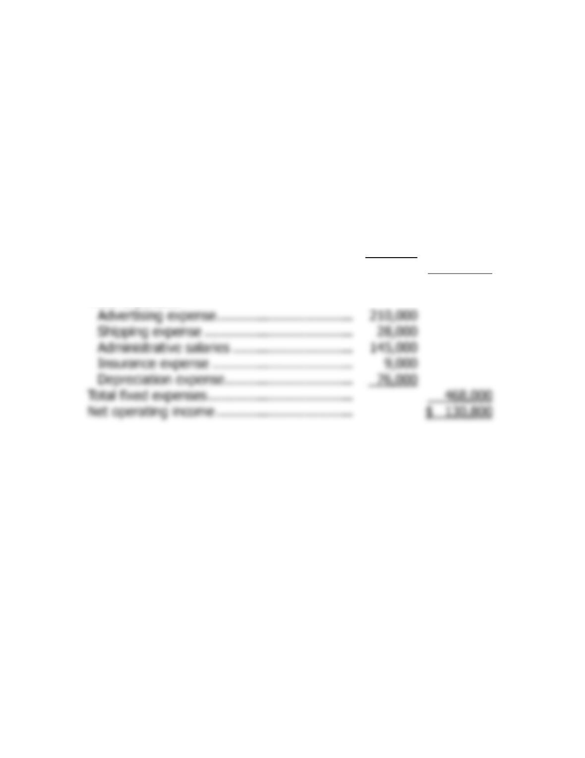
1. High-low method:
Units
Sold
Shipping
Expense
High activity level …………..
20,000
$210,000
Low activity level ……………
10,000
119,000
Change ………………………..
10,000
$91,000
Fixed cost element:
Less variable element:
Fixed cost element …………………………….
Problem 5A-9 (continued)
2.
Milden Company
Budgeted Contribution Format Income Statement
For the First Quarter, Year 3
Sales (12,000 units × $100 per unit) …………
$1,200,000
Variable expenses:
Cost of goods sold
(12,000 units × $35 unit) …………………..
$420,000
Sales commission (6% × $1,200,000) ……..
72,000
Shipping expense
(12,000 units × $9.10 per unit) …………..
109,200
Total variable expenses…………………………..
601,200
Contribution margin ………………………………
598,800
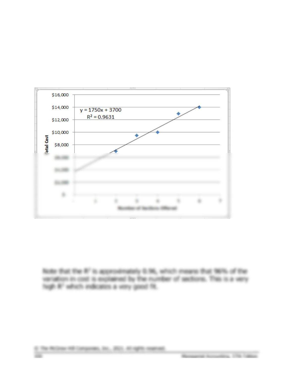
Fixed expenses:
Depreciation expense …………………………..
Net operating income …………………………….
Problem 5A-10 (30 minutes)
1. and 2.
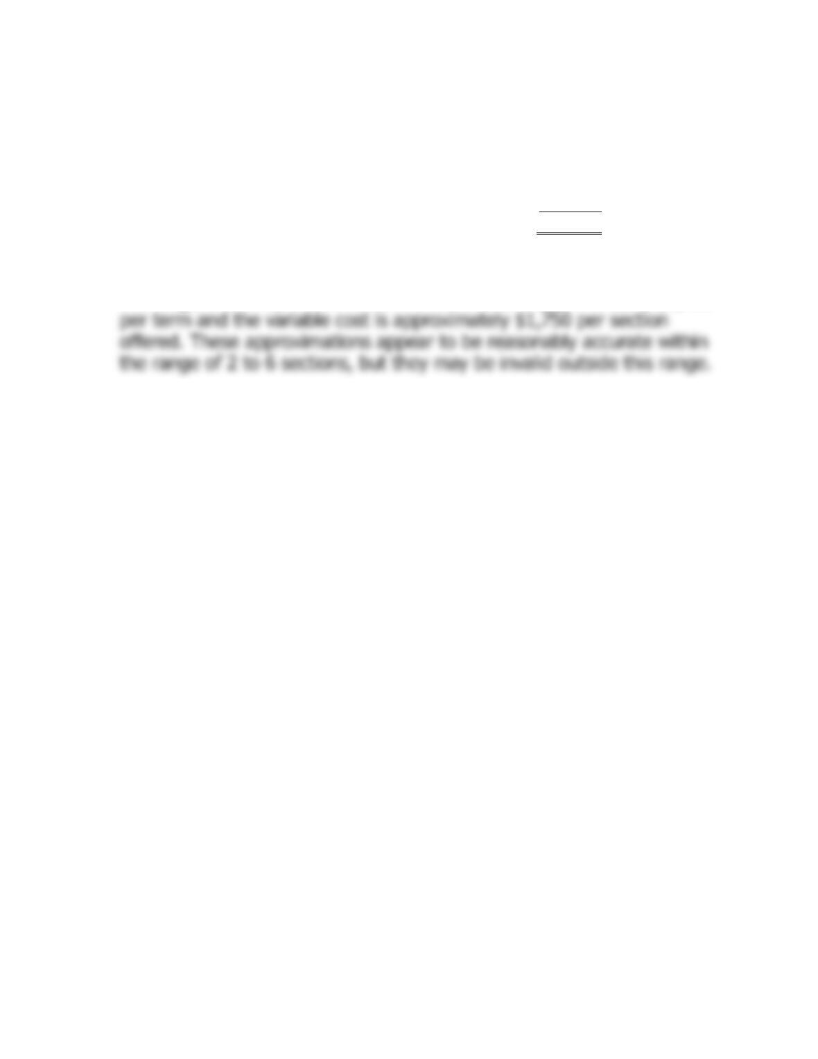
The scattergraph plot and regression estimates of fixed and variable costs
using Microsoft Excel are shown below:
The cost formula, in the form
Y
=
a
+
bX
, using number of sections
offered as the activity base is $3,700 per quarter plus $1,750 per section
offered, or:
Y = $3,700 + $1,750X
Problem 5A-10 (continued)
3. Expected total cost would be:
Fixed cost ……………………………………………….
$ 3,700
Variable cost (8 sections × $1,750 per section) .
14,000
Total cost …………………………..……………………
$17,700
The problem with using the cost formula from (2) to derive total cost is
that an activity level of 8 sections may lie outside the relevant range—
the range of activity within which the fixed cost is approximately $3,700
Case 5A-11 (60 minutes)
1. High-low method:
Hours
Cost
High level of activity …….
25,000
$99,000
Low level of activity ……..
10,000
64,500
Change ……………………..
15,000
$34,500
Variable element: $34,500 ÷ 15,000 DLH = $2.30 per MH
Fixed element:
Total cost—25,000 MH ……………………..
Fixed element …………………………………
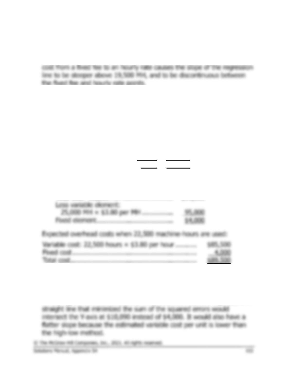
2. The scattergraph is shown below:
$70,000
$80,000
$85,000
$90,000
$95,000
$100,000
Y
Case 5A-11 (continued)
2. The scattergraph shows that there are two relevant ranges—one below
19,500 MH and one above 19,500 MH. The change in equipment lease
3. The cost formulas computed with the high-low and regression methods
are faulty since they are based on the assumption that a single straight
line provides the best fit to the data. Creating two data sets related to
the two relevant ranges will enable more accurate cost estimates.
4. High-low method:
Hours
Cost
High level of activity …….
25,000
$99,000
Low level of activity ……..
20,000
80,000
Change ……………………..
5,000
$19,000
Variable element: $19,000 ÷ 5,000 MH = $3.80 per MH
Fixed element:
Total cost—25,000 MH ……………………..
$99,000
Fixed element …………………………………
Variable cost: 22,500 hours × $3.80 per hour ………..
Fixed cost ………………………………………………………
4,000
Total cost …………………………..…………………………..
5. The high-low estimate of fixed costs is $6,090 (= $10,090 – $4,000)
lower than the estimate provided by least-squares regression. The high-
low estimate of the variable cost per machine hour is $0.27 (= $3.80 –
$3.53) higher than the estimate provided by least-squares regression. A
Case 5A-12 (45 minutes)
1. and 2.
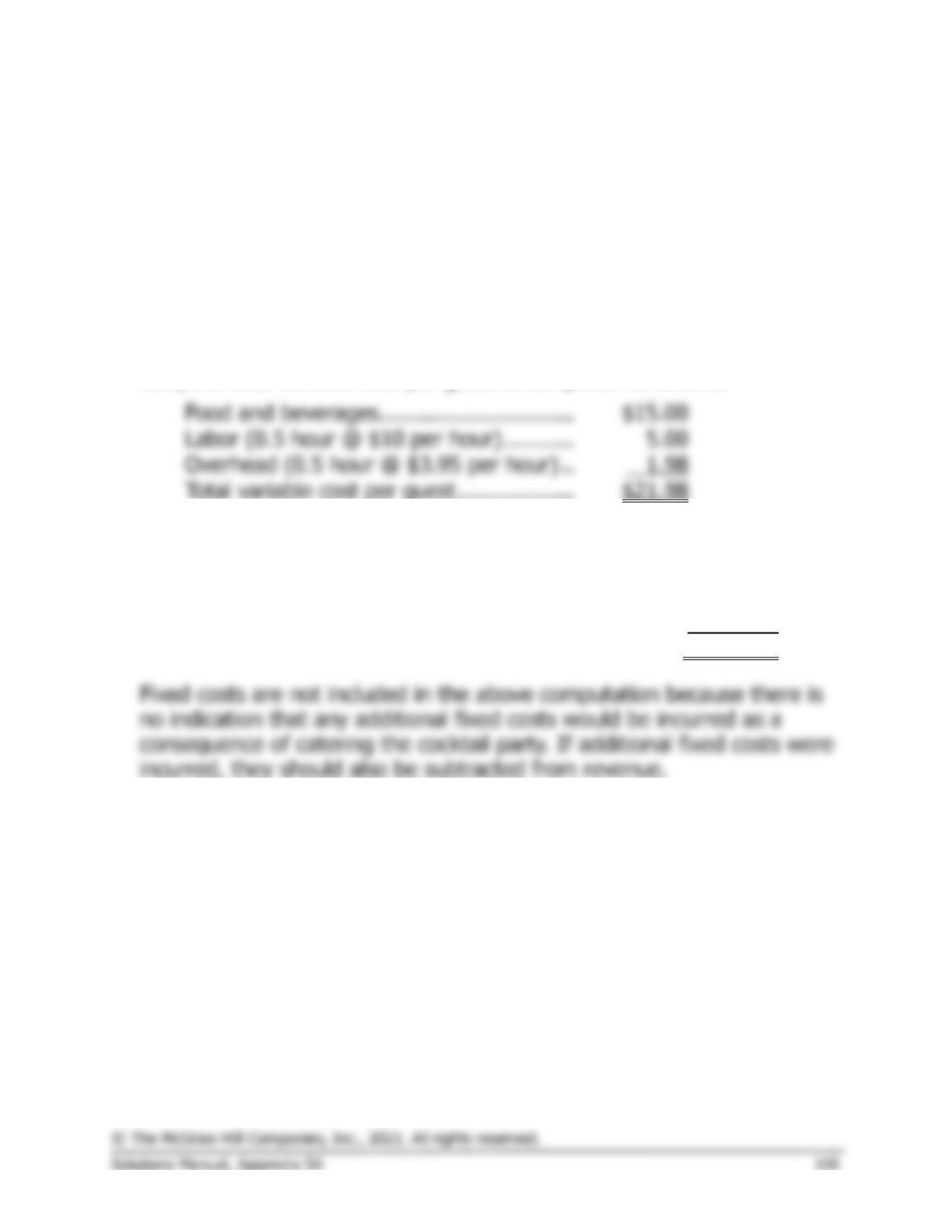
The scattergraph plot and regression estimates of fixed and variable
costs using Microsoft Excel are shown below:
The scattergraph reveals three interesting findings. First, it indicates the
relation between overhead expense and labor hours is approximated
reasonably well by a straight line. (However, there appears to be a slight
downward bend in the plot as the labor-hours increase—evidence of
increasing returns to scale. This is a common occurrence in practice. See
Noreen & Soderstrom, “Are overhead costs strictly proportional to
activity?”
Journal of Accounting and Economics
, vol. 17, 1994, pp. 255-
278.)
Second, the data points are all fairly close to the straight line. This
indicates that most of the variation in overhead expenses is explained by
labor hours. As a consequence, there probably wouldn’t be much benefit
to investigating other possible cost drivers for the overhead expenses.
CASE 5A-12 (continued)
The cost formula, in the form
Y
=
a
+
bX
, using labor-hours as the
activity base is $48,126 per month plus $3.95 per labor-hour, or:
Y = $48,126 + $3.95X
Note that the R2 is approximately 0.96, which means that 96% of the
variation in cost is explained by labor-hours. This is a very high R2 which
indicates a very good fit.
3. Using the least-squares regression estimate of the variable overhead
cost, the total variable cost per guest is computed as follows:
Food and beverages…………………………
Labor (0.5 hour @ $10 per hour) ………..
Overhead (0.5 hour @ $3.95 per hour) ..
Total variable cost per guest ………………
The total contribution from 180 guests paying $31 each is computed as
follows:
Sales (180 guests @ $31.00 per guest) …………..
$5,580.00
Variable cost (180 guests @ $21.98 per guest) …
3,956.40
Contribution to profit ………………………………….
$1,623.60
4. Assuming that no additional fixed costs are incurred as a result of
catering the charity event, any price greater than the variable cost per
guest of roughly $22 would contribute to profits.
CASE 5A-12 (continued)
5. We would favor bidding slightly less than $30 to get the contract. Any
bid above $22 would contribute to profits and a bid at the normal price
of $31 is unlikely to land the contract. And apart from the contribution
to profit, catering the event would show off the company’s capabilities
to potential clients. The danger is that a price that is lower than the
normal bid of $31 might set a precedent for the future or it might