Chapter 5
Cost-Volume-Profit Relationships
Solutions to Questions
5-1 The contribution margin (CM) ratio is
the ratio of the total contribution margin to total
sales revenue. It can also be expressed as the
ratio of the contribution margin per unit to the
selling price per unit. It is used in target profit
and break-even analysis and can be used to
quickly estimate the effect on profits of a
change in sales revenue.
5-2 Incremental analysis focuses on the
changes in revenues and costs that will result
from a particular action.
5-3 All other things equal, Company B, with
its higher fixed costs and lower variable costs,
will have a higher contribution margin ratio than
Company A. Therefore, it will tend to realize a
larger increase in contribution margin and in
profits when sales increase.
higher unit volume. (b) If the fixed cost
increased, then both the fixed cost line and the
total cost line would shift upward and the break-
even point would occur at a higher unit volume.
(c) If the variable cost per unit increased, then
the total cost line would rise more steeply and
the break-even point would occur at a higher
unit volume.
5-7 The margin of safety is the excess of
budgeted (or actual) sales over the break-even
volume of sales. It is the amount by which sales
can drop before losses begin to be incurred.
5-8 The sales mix is the relative proportions
in which a company’s products are sold. The
usual assumption in cost-volume-profit analysis
is that the sales mix will not change.
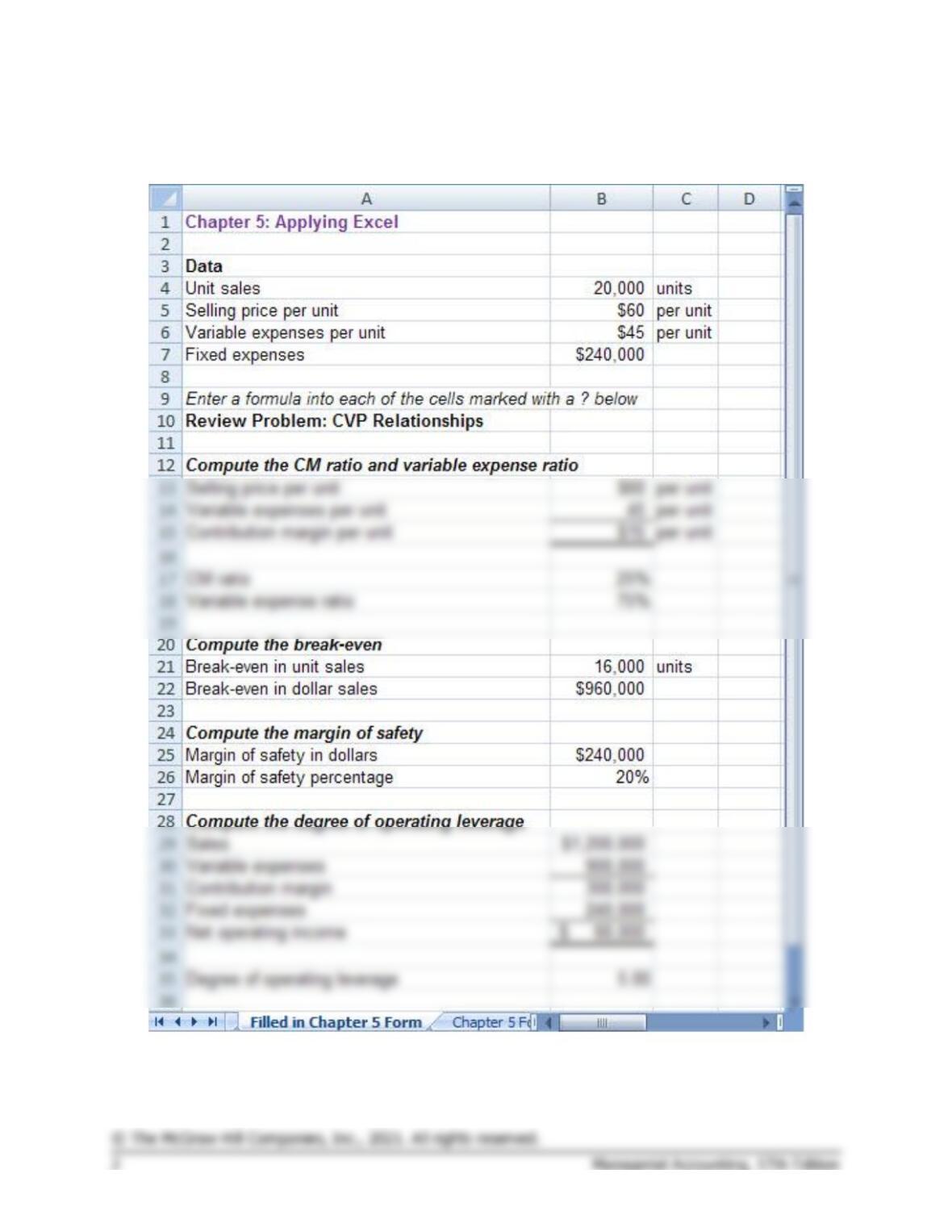
Chapter 5: Applying Excel
The completed worksheet is shown below.
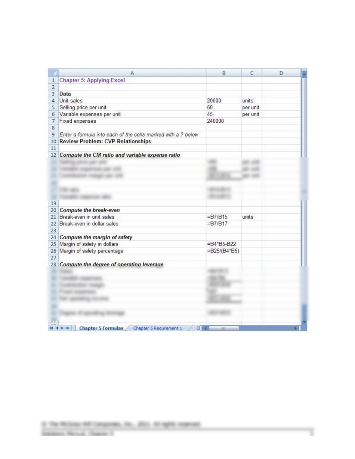
Chapter 5: Applying Excel (continued)
The completed worksheet, with formulas displayed, is shown below.
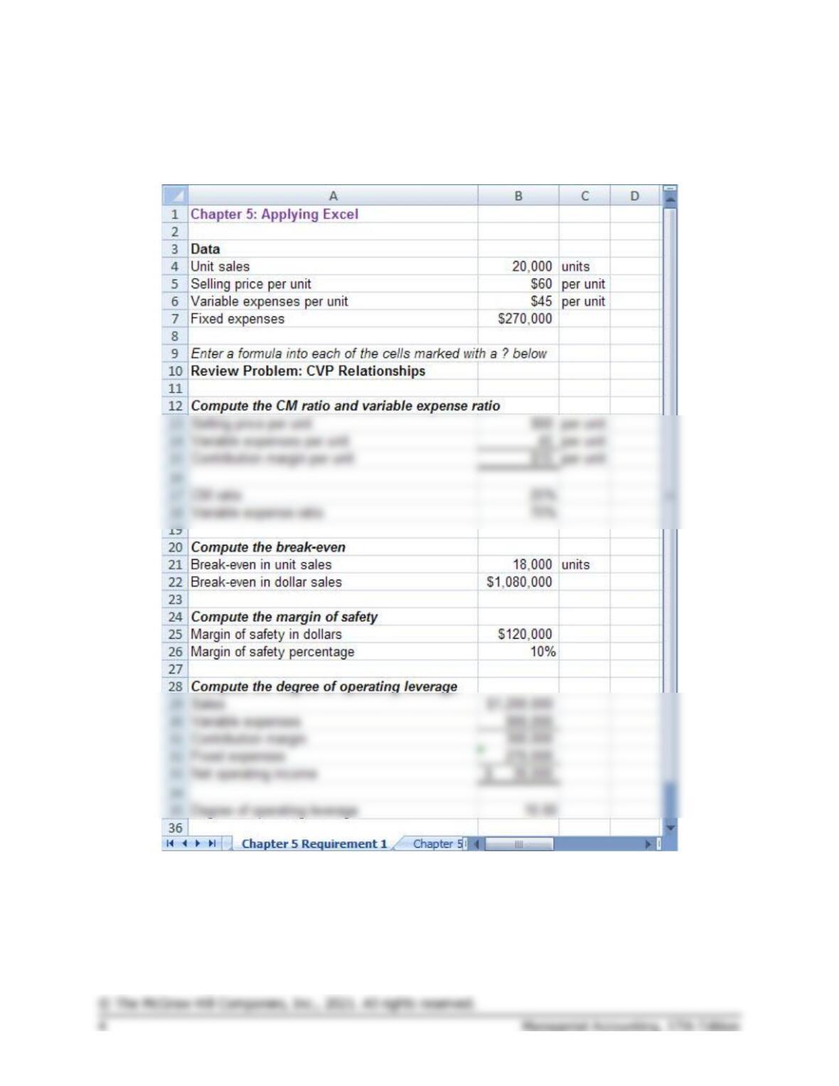
Chapter 5: Applying Excel (continued)
1. When the fixed expenses are changed to $270,000, the worksheet
changes as shown below:
The margin of safety percentage is now 10%, whereas it was 20%
before. This change occurred because the increase in fixed expenses
increased the break-even point and hence reduced the margin of safety
available for the current level of unit sales.
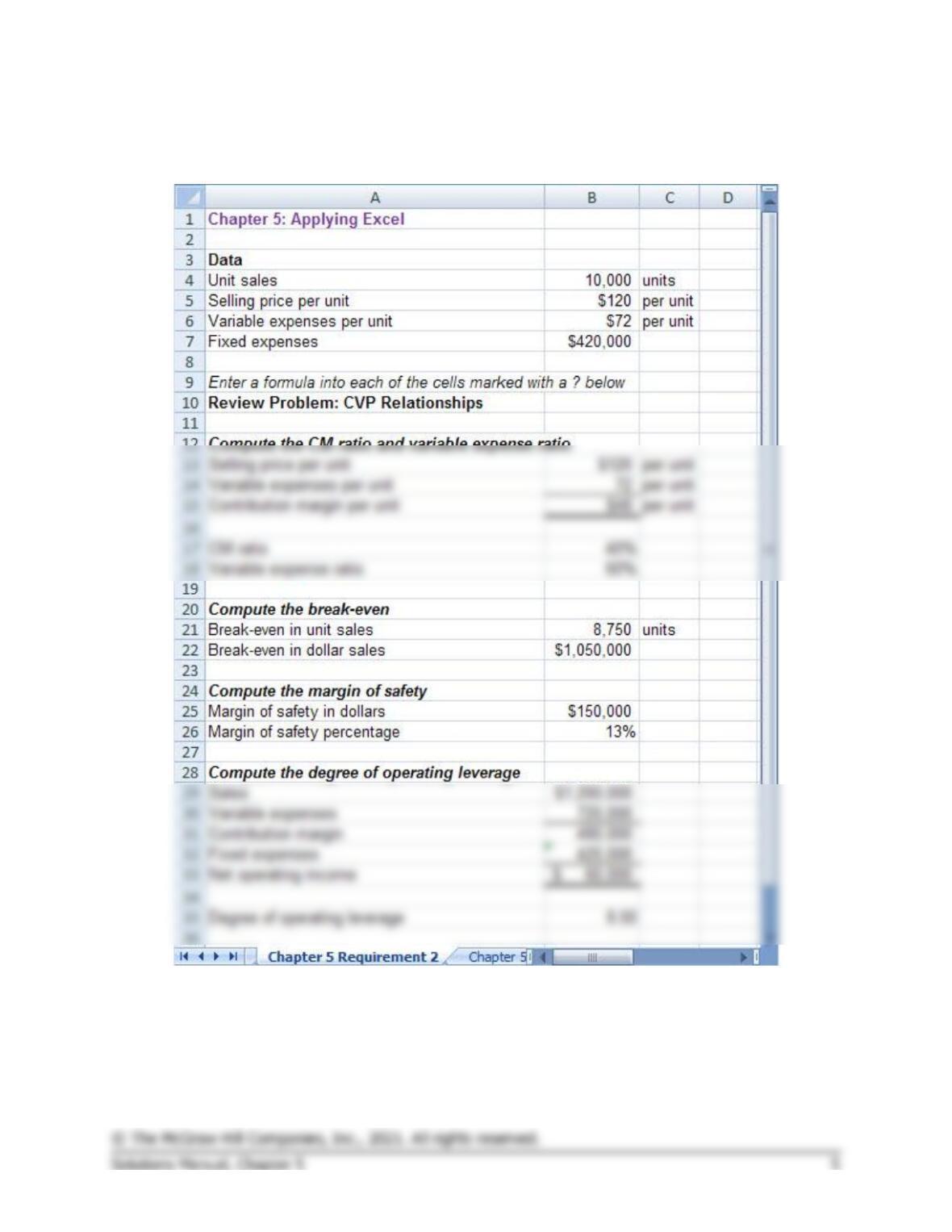
Chapter 5: Applying Excel (continued)
2. With the changes in the data, the worksheet should look like this:
The margin of safety percentage is 13% and the degree of operating
leverage is 8.
Chapter 5: Applying Excel (continued)
3. The degree of operating leverage can be used to estimate the expected
percentage increase in net operating income from a 15% increase in
unit sales as follows:
Percentage change in net operating income = Degree of operating
leverage × Percentage change in sales = 8.00 × 15% = 120%
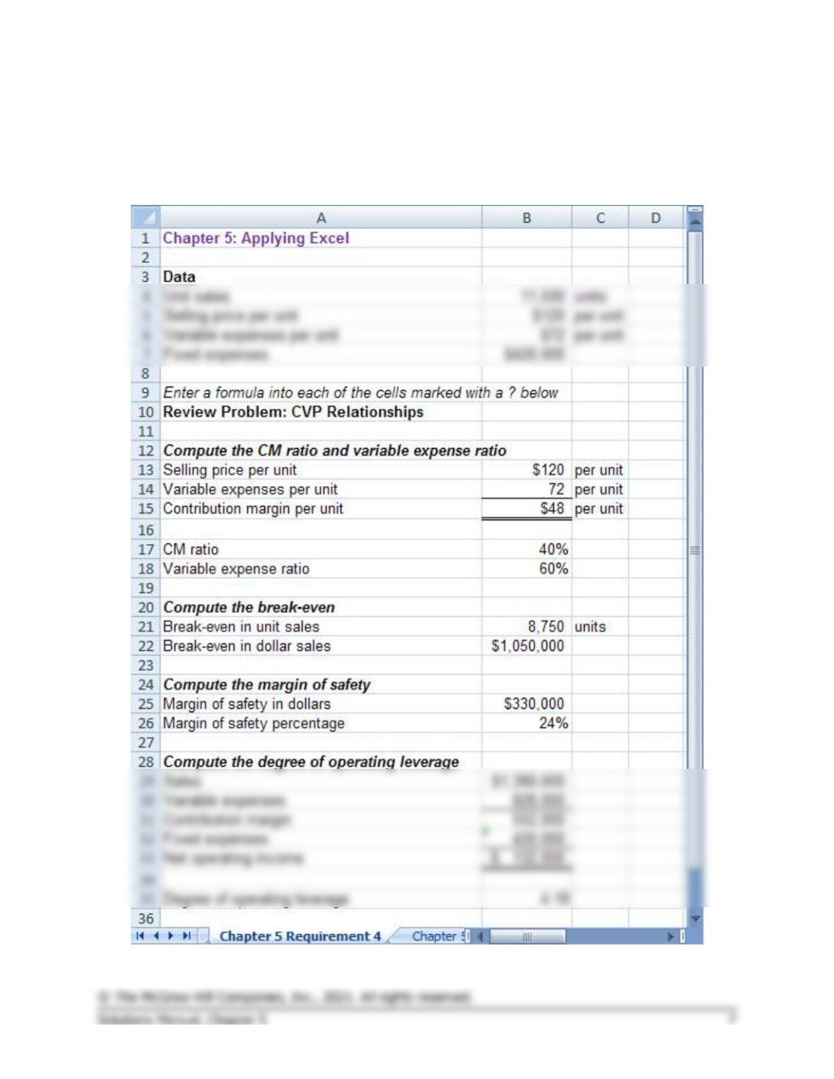
Chapter 5: Applying Excel (continued)
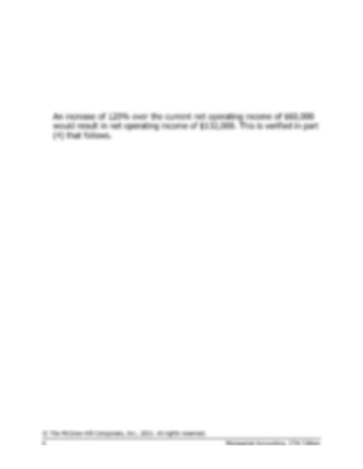
4. Increasing the unit sales by 15% results in net operating income of
$132,000—an increase of 120% over the previous net operating income
of $60,000.
Chapter 5: Applying Excel (continued)
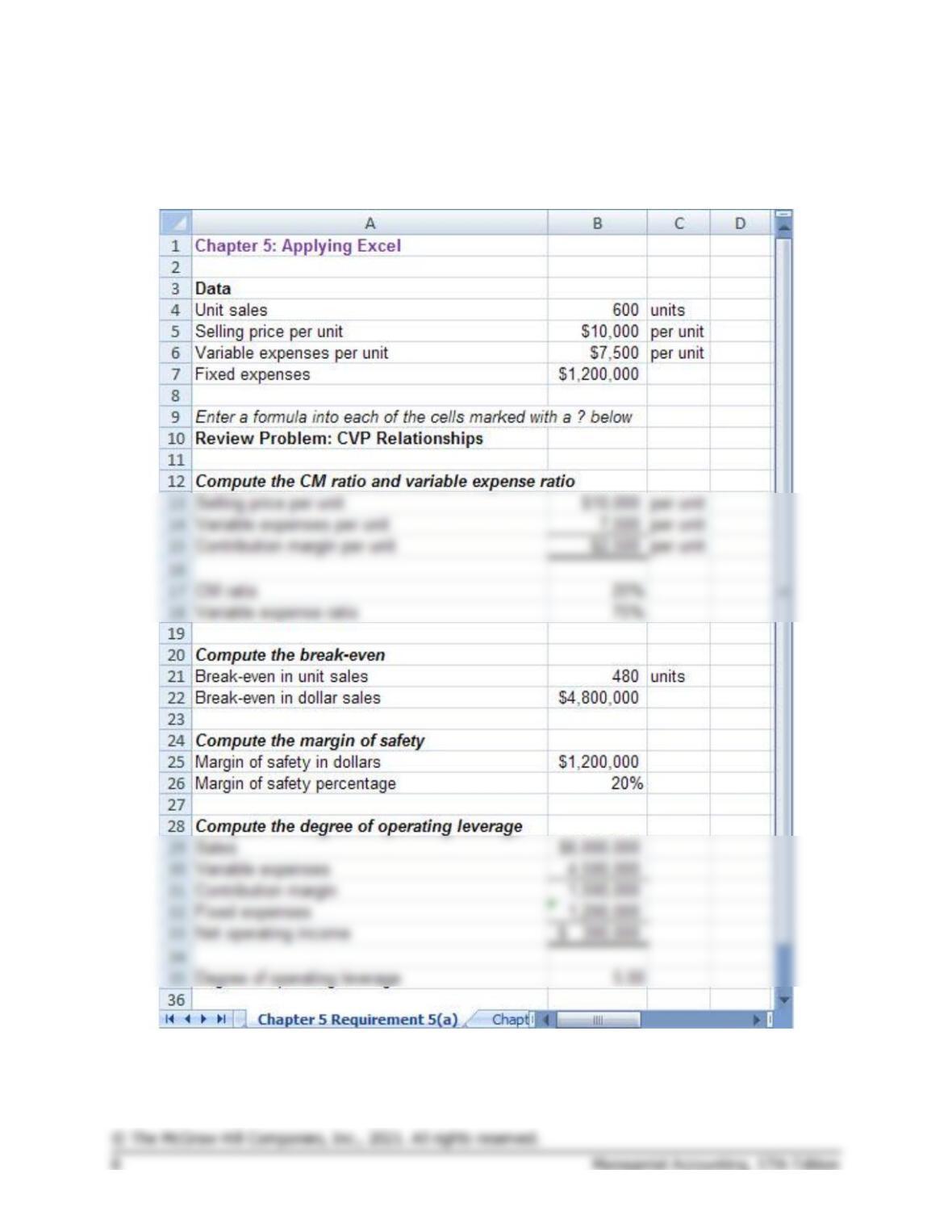
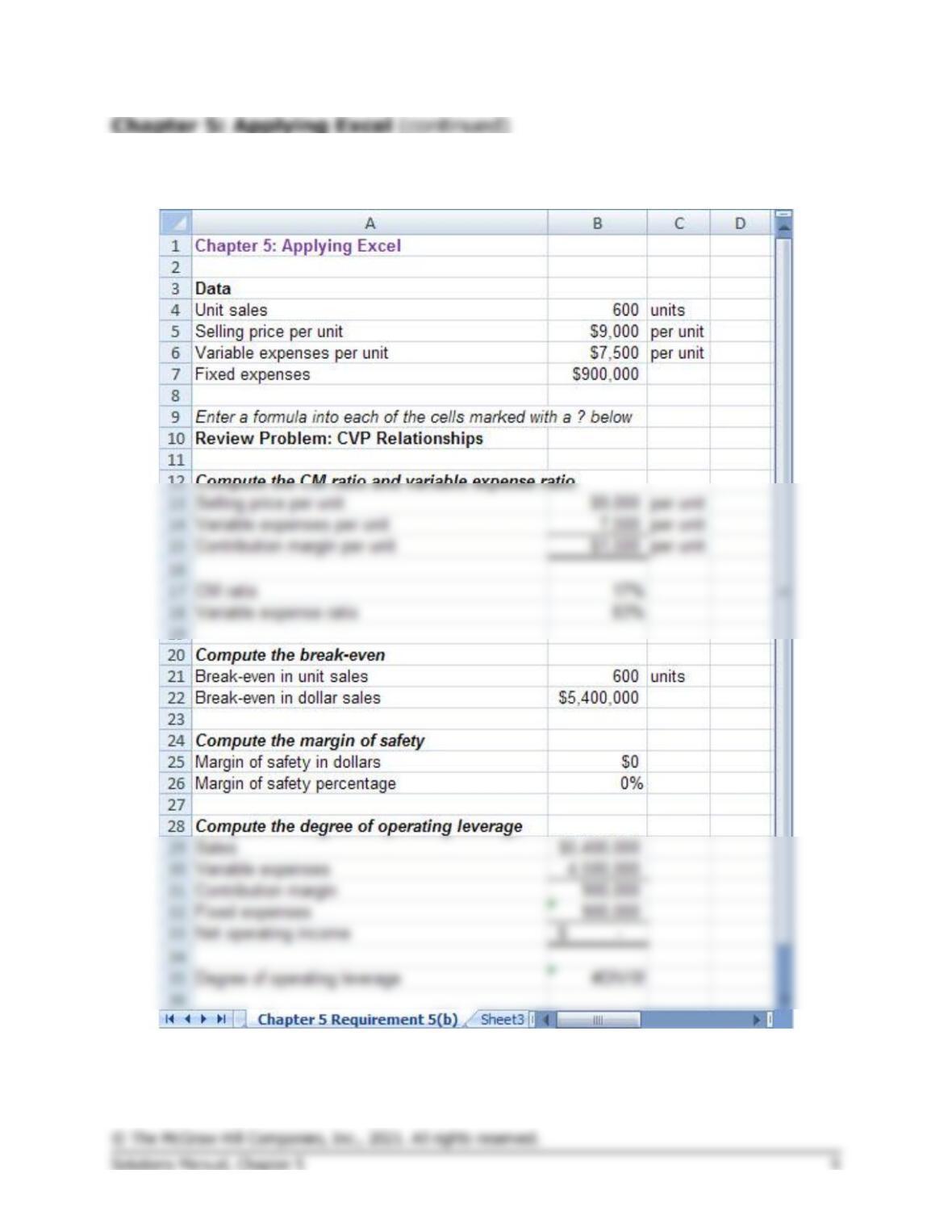
5. a. The initial plan for the Western Hombre motorcycle is summarized
below:
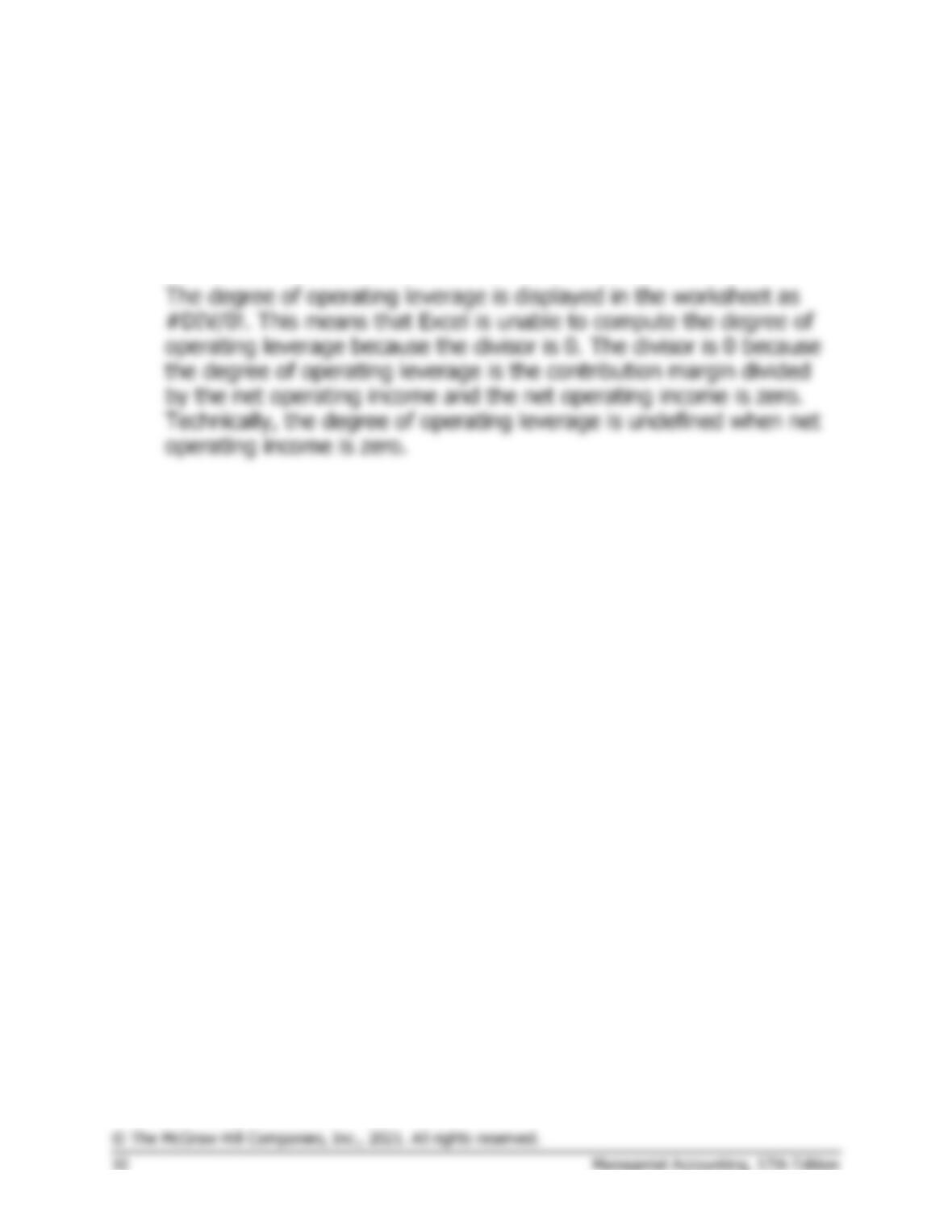
5. b. The modified plan for the Western Hombre motorcycle is summarized
below:
Chapter 5: Applying Excel (continued)
This does not appear to be a good plan. At best, Thad would only
break even—and that assumes that 600 units would still be sold
despite the drastic reduction in advertising expenses. The margin of
safety is zero which means that any decrease in sales to below 600
units would result in a loss.
1. The contribution margin per unit is calculated as follows:
Total contribution margin (a) …………..
$8,000
Total units sold (b) ………………………..
1,000
units
Contribution margin per unit (a) ÷ (b) .
$8.00
per unit
2. The contribution margin ratio is calculated as follows:
Total contribution margin (a) …………..
$8,000
Total sales (b) ………………………………
$20,000
Contribution margin ratio (a) ÷ (b) ……
40%
3. The variable expense ratio is calculated as follows:
Total variable expenses (a) ……………..
$12,000
Total sales (b) ………………………………
$20,000
Variable expense ratio (a) ÷ (b) ……….
60%
4. The increase in net operating income is calculated as follows:
Contribution margin per unit (a) ……………….
per unit
Increase in unit sales (b) ……………………….
unit
Increase in net operating income (a) × (b) ..
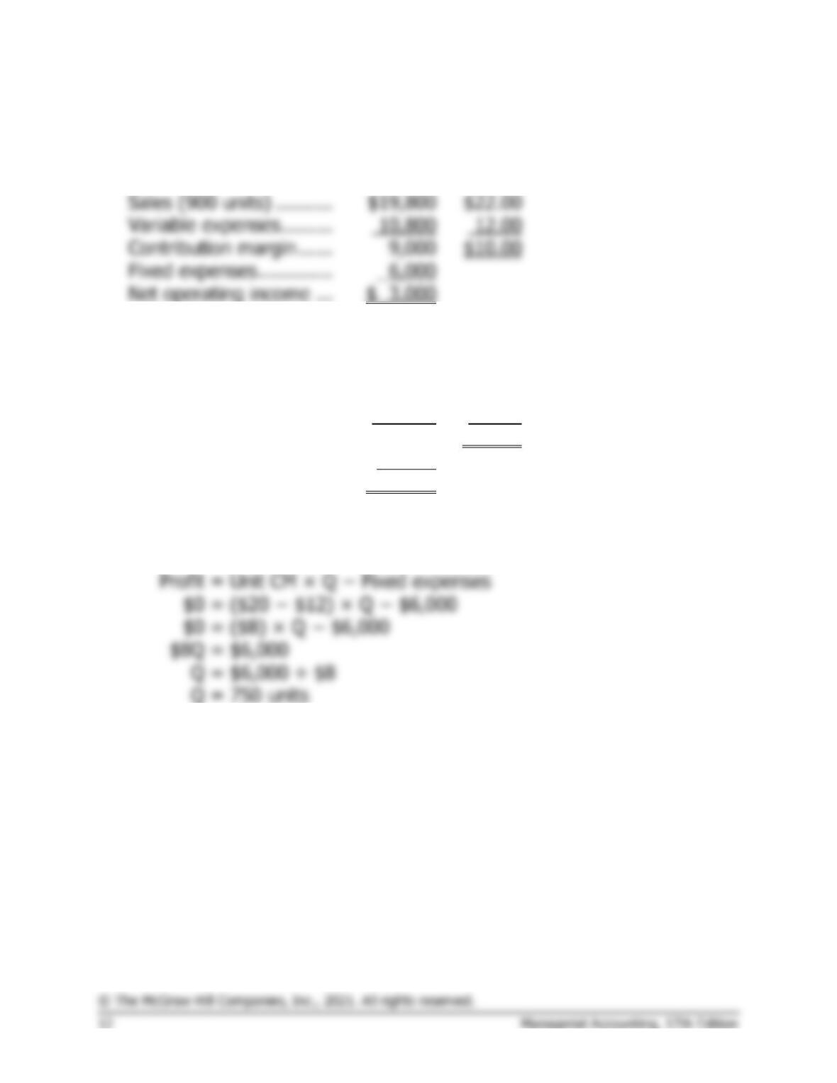
5. If sales decline to 900 units, the net operating income would be
computed as follows:
Total
Per Unit
Sales (900 units) ……….
$18,000
$20.00
Variable expenses ………
10,800
12.00
Contribution margin ……
7,200
$ 8.00
Fixed expenses ………….
6,000
Net operating income …
$ 1,200
The Foundational 15 (continued)
6. The new net operating income would be computed as follows:
Total
Per Unit
Sales (900 units) ……….
$19,800
$22.00
Variable expenses ………
Contribution margin ……
Fixed expenses ………….
Net operating income …
7. The new net operating income would be computed as follows:
Total
Per Unit
Sales (1,250 units) …….
$25,000
$20.00
Variable expenses ………
16,250
13.00
Contribution margin ……
8,750
$ 7.00
Fixed expenses ………….
7,500
Net operating income …
$ 1,250
8. The equation method yields the break-even point in unit sales, Q, as
follows:
= Unit CM × Q − Fixed expenses
= ($20 − $12) × Q − $6,000
= ($8) × Q − $6,000
= $6,000
= $6,000 ÷ $8
= 750 units
9. The equation method yields the dollar sales to break-even as follows:
Profit
= CM ratio × Sales − Fixed expenses
$0
= 0.40 × Sales − $6,000
0.40 × Sales
= $6,000
Sales
= $6,000 ÷ 0.40
Sales
= $15,000
The dollar sales to break-even ($15,000) can also be computed by
multiplying the selling price per unit ($20) by the unit sales to break-
even (750 units).
The Foundational 15 (continued)
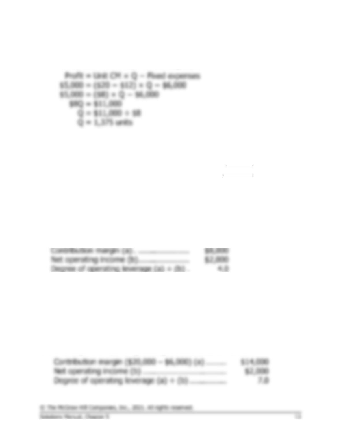
10. The equation method yields the target profit as follows:
= Unit CM × Q − Fixed expenses
= ($20 − $12) × Q − $6,000
= ($8) × Q − $6,000
= $11,000
= $11,000 ÷ $8
= 1,375 units
11. The margin of safety in dollars is calculated as follows:
Sales ……………………………………………………..
$20,000
Break-even sales (at 750 units) ……………………
15,000
Margin of safety (in dollars) ………………………..
$ 5,000
The margin of safety as a percentage of sales is calculated as follows:
Margin of safety (in dollars) (a) ……………..
$5,000
Sales (b) …………………………………………..
$20,000
Margin of safety percentage (a) ÷ (b) …….
25%
12. The degree of operating leverage is calculated as follows:
Contribution margin (a) . ………………….
$8,000
Net operating income (b) ………………….
$2,000
Degree of operating leverage (a) ÷ (b) .
13. A 5% increase in unit sales should result in a 20% increase in net
operating income, computed as follows:
Degree of operating leverage (a) ………………………..
4.0
Percent increase in sales (b) ………………………………
5%
Percent increase in net operating income (a) × (b) …
20%
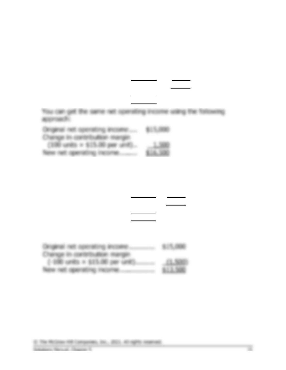
14. The degree of operating leverage is calculated as follows:
Contribution margin ($20,000 – $6,000) (a) ………
Net operating income (b) ………………………………
$2,000
Degree of operating leverage (a) ÷ (b) …………….

The Foundational 15 (continued)
15. A 5% increase in unit sales should result in a 35% increase in net
operating income, computed as follows:
Degree of operating leverage (a) …………………………
7.0
Percent increase in sales (b) ……………………………….
5%
Percent increase in net operating income (a) × (b) ….
35%
Exercise 5-1 (20 minutes)
1. The revised net operating income would be:
Total
Per Unit
Sales (10,100 units) ……..
$353,500
$35.00
Variable expenses ………..
202,000
20.00
Contribution margin ……..
151,500
$15.00
Fixed expenses ……………
135,000
Net operating income ……
$ 16,500
Original net operating income ….
$15,000
1,500
New net operating income ………
$16,500
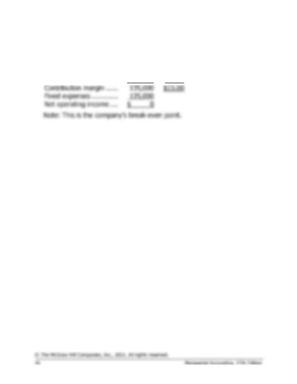
2. The revised net operating income would be:
Total
Per Unit
Sales (9,900 units) …………
$346,500
$35.00
Variable expenses ………….
198,000
20.00
Contribution margin ……….
148,500
$15.00
Fixed expenses ……………..
135,000
Net operating income ……..
$ 13,500
You can get the same net operating income using the following
approach:
Original net operating income ………….
$15,000
New net operating income ………………
$13,500
Exercise 5-1 (continued)
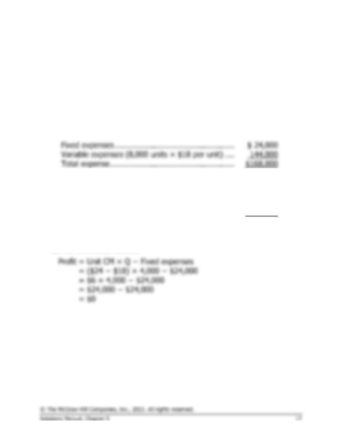
3. The revised net operating income would be:
Total
Per Unit
Sales (9,000 units) ……..
$315,000
$35.00
Variable expenses ………
180,000
20.00
Contribution margin ……
Fixed expenses ………….
Net operating income ….
Exercise 5-2 (30 minutes)
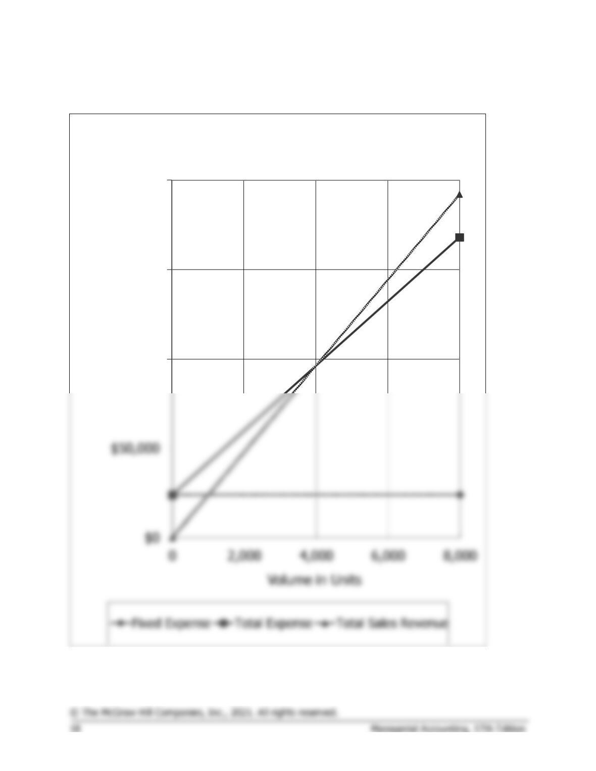
1. The CVP graph can be plotted using the three steps outlined in the text.
The graph appears on the next page.
Step 1. Draw a line parallel to the volume axis to represent the total
fixed expense. For this company, the total fixed expense is $24,000.
Step 2. Choose some volume of sales and plot the point representing
total expenses (fixed and variable) at the activity level you have
selected. We’ll use the sales level of 8,000 units.
Step 3. Choose some volume of sales and plot the point representing
total sales dollars at the activity level you have selected. We’ll use the
sales level of 8,000 units again.
Total sales revenue (8,000 units × $24 per unit) ..
$192,000
2. The break-even point is the point where the total sales revenue and the
total expense lines intersect. This occurs at sales of 4,000 units. This
= $0
Exercise 5-2 (continued)
$100,000
$150,000
$200,000
Dollars
CVP Graph
Exercise 5-3 (15 minutes)
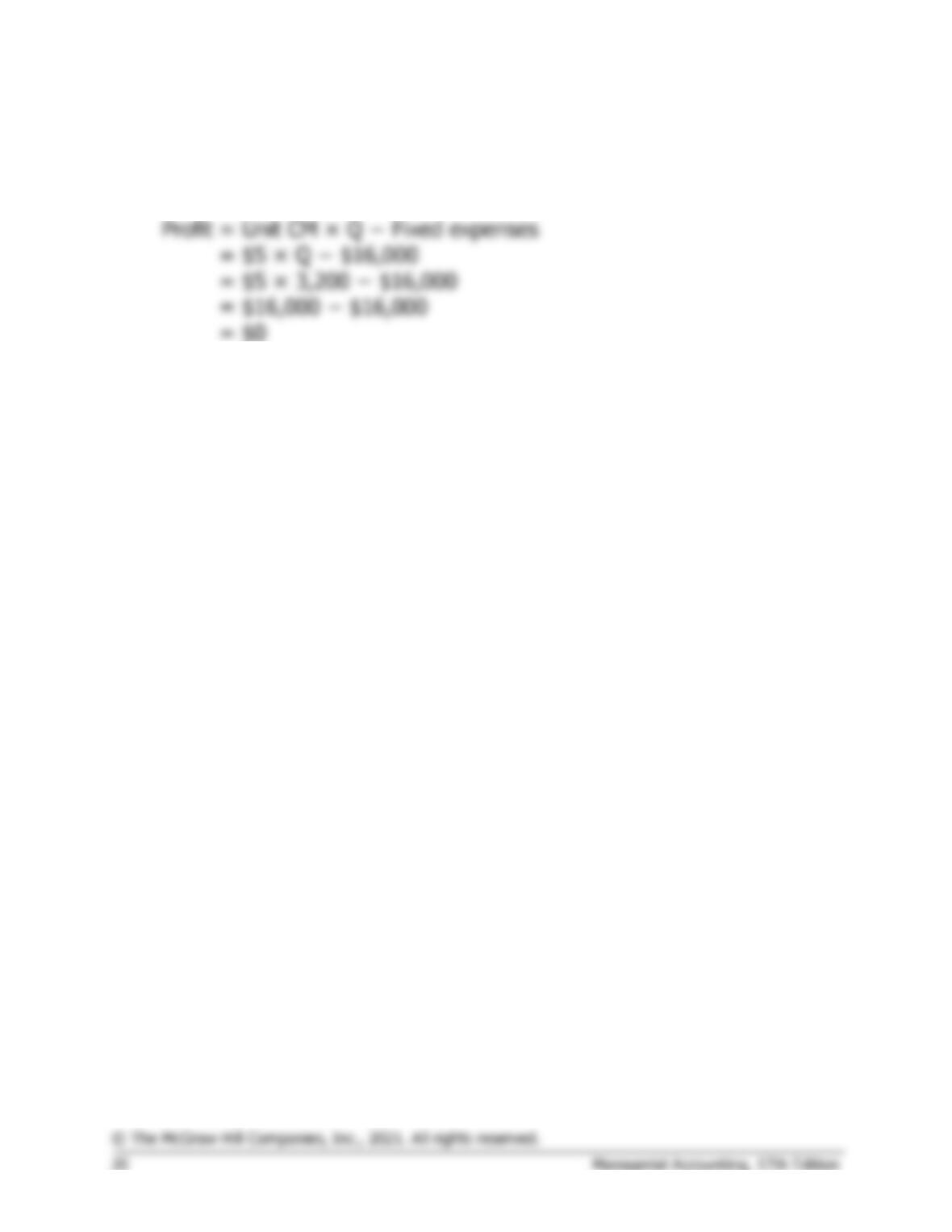
1. The profit graph is based on the following simple equation:
Profit
= Unit CM × Q − Fixed expenses
Profit
= ($16 − $11) × Q − $16,000
Profit
= $5 × Q − $16,000
To plot the graph, select two different levels of sales such as Q = 0 and
Q = 4,000. The profit at these two levels of sales are -$16,000 (= $5 ×
0 − $16,000) and $4,000 (= $5 × 4,000 − $16,000).
$0
$5,000
Profit Graph
Exercise 5-3 (continued)
2. Looking at the graph, the break-even point appears to be 3,200 units.
This can be verified as follows: