Problem 5-31 (continued)
2.
a.
Line 3:
Remain unchanged.
Line 9:
Have a steeper slope.
Break-even point:
Decrease.
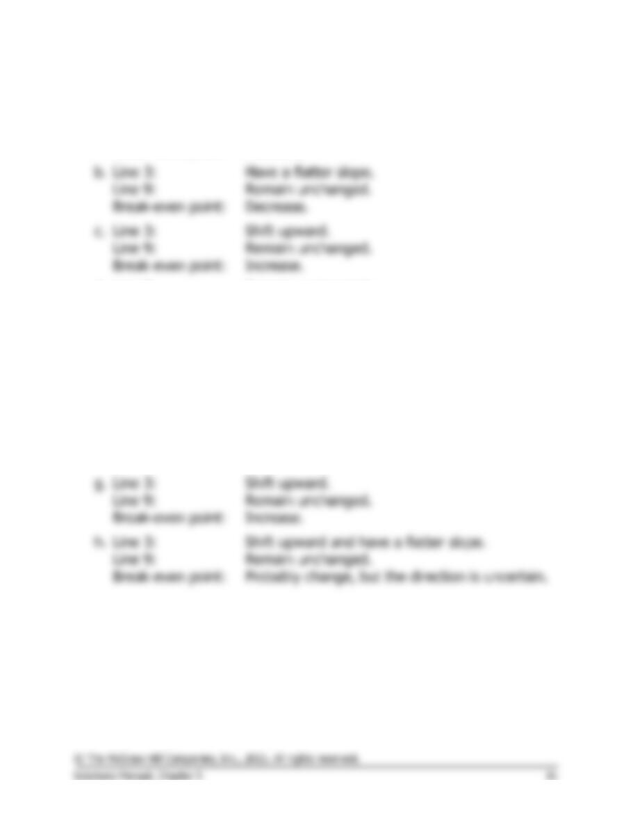
b.
Line 3:
Have a flatter slope.
Line 9:
Remain unchanged.
Break-even point:
Decrease.
Line 3:
Shift upward.
Line 9:
Remain unchanged.
Break-even point:
Increase.
d.
Line 3:
Remain unchanged.
Line 9:
Remain unchanged.
Break-even point:
Remain unchanged.
e.
Line 3:
Shift downward and have a steeper slope.
Line 9:
Remain unchanged.
Break-even point:
Probably change, but the direction is uncertain.
f.
Line 3:
Have a steeper slope.
Line 9:
Have a steeper slope.
Break-even point:
Remain unchanged in terms of units; increase
in terms of total dollars of sales.
g.
Line 3:
Shift upward.
Line 9:
Remain unchanged.
Break-even point:
Increase.
Line 3:
Shift upward and have a flatter slope.
Line 9:
Remain unchanged.
Break-even point:
Probably change, but the direction is uncertain.
Case 5-32 (75 minutes)
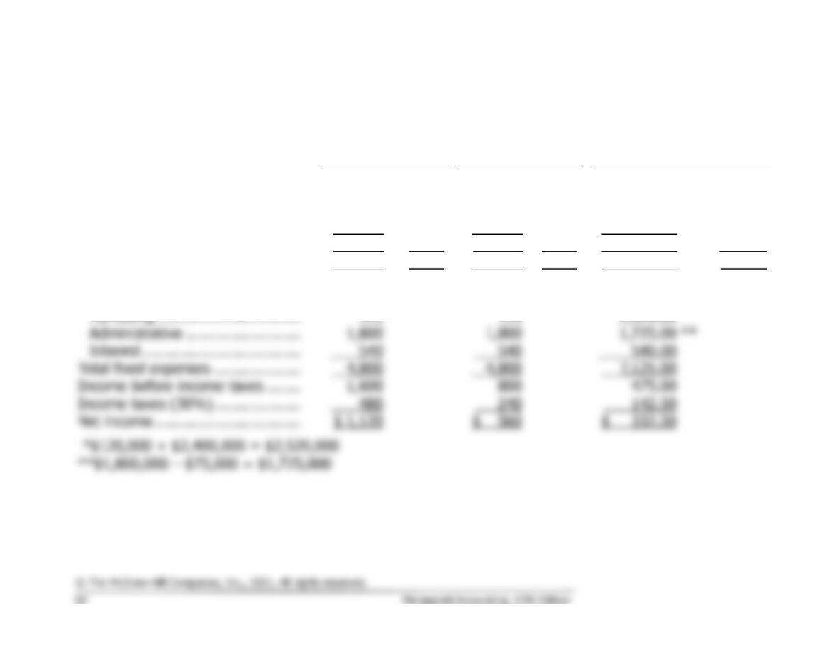
Before proceeding with the solution, it is helpful first to restructure the data into contribution format for
each of the three alternatives. (The data in the statements below are in thousands.)
15% Commission
20% Commission
Own Sales Force
Sales ……………………………………
$16,000
100%
$16,000
100%
$16,000.00
100.0%
Variable expenses:
Manufacturing ……………………..
7,200
7,200
7,200.00
Commissions (15%, 20%, 7.5%)
2,400
3,200
1,200.00
Total variable expenses …………….
9,600
60%
10,400
65%
8,400.00
52.5%
Contribution margin …………………
6,400
40%
5,600
35%
7,600.00
47.5%
Fixed expenses:
Manufacturing overhead …………
2,340
2,340
2,340.00
Marketing …………………………...
2,520.00
*
Interest ………………………………
540
540.00
Total fixed expenses ………………..
4,800
4,800
7,125.00
Income before income taxes ……..
Income taxes (30%) ………………..
142.50
Net income …………………………...
$ 1,120
*$120,000 + $2,400,000 = $2,520,000
**$1,800,000 – $75,000 = $1,725,000
Case 5-32 (continued)
1. When the income before taxes is zero, income taxes will also be zero
and net income will be zero. Therefore, the break-even calculations can
be based on the income before taxes.
a. Break-even point in dollar sales if the commission remains 15%:
Fixed expenses $4,800,000
Dollar sales to = = = $12,000,000
break even CM ratio 0.40
b. Break-even point in dollar sales if the commission increases to 20%:
Fixed expenses $4,800,000
Dollar sales to = = = $13,714,286
break even CM ratio 0.35
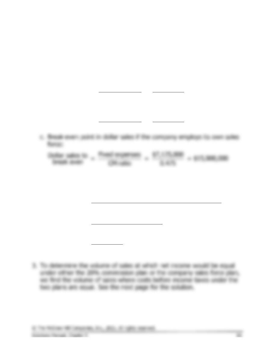
Fixed expenses $7,125,000
Dollar sales to = = = $15,000,000
break even CM ratio 0.475
2. In order to generate a $1,120,000 net income, the company must
generate $1,600,000 in income before taxes. Therefore,
Target income before taxes + Fixed expenses
Dollar sales to =
attain target CM ratio
$1,600,000 + $4,800,000
=
0.35
$6,400,000
= = $18,285,714
0.35
Case 5-32 (continued)
X =
Total sales revenue
0.65X + $4,800,000 =
0.525X + $7,125,000
0.125X =
$2,325,000
X =
$2,325,000 ÷ 0.125
X =
$18,600,000
Thus, at a sales level of $18,600,000 either plan would yield the same
income before taxes and net income. Below this sales level, the
commission plan would yield the largest net income; above this sales
level, the sales force plan would yield the largest net income.
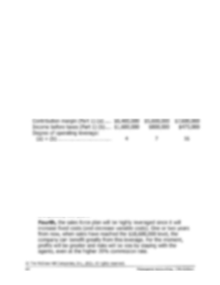
4. a., b., and c.
15%
Commission
20%
Commission
Own
Sales Force
Contribution margin (Part 1) (a) …..
Income before taxes (Part 1) (b) ….
5. We would continue to use the sales agents for at least one more year,
and possibly for two more years. The reasons are as follows:
First, use of the sales agents would have a less dramatic effect on
net income.
Second, use of the sales agents for at least one more year would
give the company more time to hire competent people and get the
sales group organized.
Third, the sales force plan doesn’t become more desirable than the
use of sales agents until the company reaches sales of $18,600,000 a
year. This level probably won’t be reached for at least one more year,
Appendix 5A
Analyzing Mixed Costs
Exercise 5A-1 (20 minutes)
1.
Occupancy-
Days
Electrical
Costs
High activity level (August) ..
2,406
$5,148
Low activity level (October) .
124
1,588
Change ………………………….
2,282
$3,560
Variable cost = Change in cost ÷ Change in activity
= $3,560 ÷ 2,282 occupancy-days
= $1.56 per occupancy-day
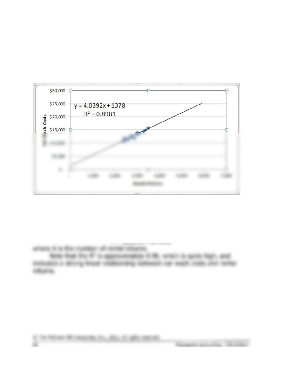
2. Electrical costs may reflect seasonal factors other than just the variation
in occupancy days. For example, common areas such as the reception
area must be lighted for longer periods during the winter than in the
summer. This will result in seasonal fluctuations in the fixed electrical
Total cost (August)……………………………………………..
Fixed cost element ……………………………………………..
Exercise 5A-2 (20 minutes)
1. and 2.
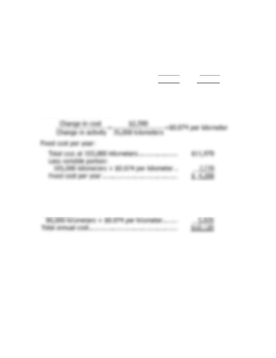
The scattergraph plot and least-squares regression estimates of fixed and
variable costs using Microsoft Excel are shown below:
The intercept provides the estimate of the fixed cost element, $1,378 per
month, and the slope provides the estimate of the variable cost element,
$4.04 per rental return. Expressed as an equation in the form
Y
=
a
+
bX
,
the relation between car wash costs and rental returns is
Exercise 5A-3 (20 minutes)
1.
Kilometers
Driven
Total Annual
Cost*
High level of activity …………………….
105,000
$11,970
Low level of activity ……………………..
70,000
9,380
Change ……………………………………..
35,000
$ 2,590
*
105,000 kilometers × $0.114 per kilometer = $11,970
70,000 kilometers × $0.134 per kilometer = $9,380
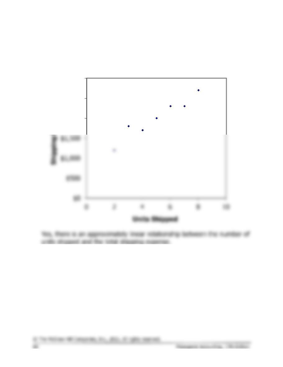
Variable cost per kilometer:
Total cost at 105,000 kilometers …………………
Fixed cost per year ………………………………….
$ 4,200
2. Y = $4,200 + $0.074X
3.
Fixed cost …………………………..…………………….
$ 4,200
Total annual cost ………………………………………..
Variable cost:
Exercise 5A-4 (45 minutes)
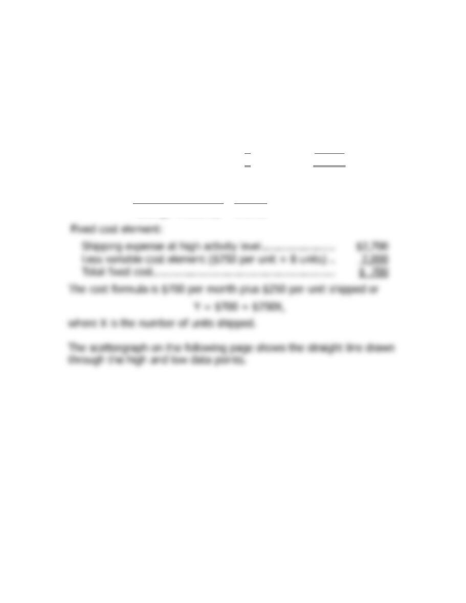
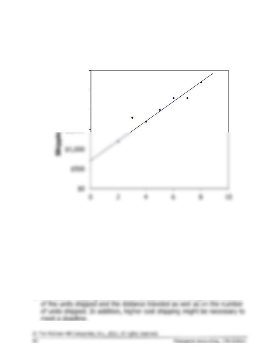
1. The scattergraph appears below:
$2,000
$2,500
$3,000
Exercise 5A-4 (continued)
2. The high-low estimates and cost formula are computed as follows:
Units Shipped
Shipping Expense
High activity level (June) …..
8
$2,700
Low activity level (July) …….
2
1,200
Change ………………………….
6
$1,500
Variable cost element:
Change in expense $1,500
= =$250 per unit.
Change in activity 6 units
Shipping expense at high activity level …………………..
Less variable cost element ($250 per unit × 8 units) ..
Total fixed cost …………………………………………………
Exercise 5A-4 (continued)
3. The high-low estimate of fixed costs is $210.71 (= $910.71 – $700.00)
lower than the estimate provided by least-squares regression. The high-
low estimate of the variable cost per unit is $32.14 (= $250.00 –
$217.86) higher than the estimate provided by least-squares regression.
A straight line that minimized the sum of the squared errors would
intersect the Y-axis at $910.71 instead of $700. It would also have a
flatter slope because the estimated variable cost per unit is lower than
the high-low method.
$2,000
$2,500
$3,000
Units Shipped
Exercise 5A-5 (20 minutes)
1. and 2.
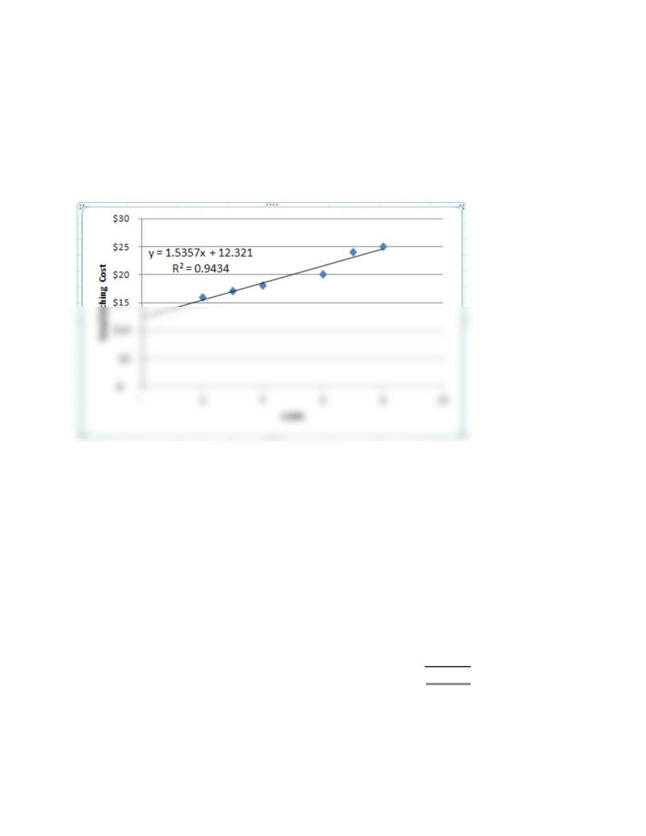
The scattergraph plot and regression estimates of fixed and variable
costs using Microsoft Excel are shown below:
Note that the R2 is approximately 0.94, which means that 94% of the
variation in etching costs is explained by the number of units etched.
This is a very high R2 which indicates a very good fit.
The regression equation, in the form
Y
=
a
+
bX,
is as follows (where
a
is rounded to nearest dollar and
b
is rounded to the nearest cent):
Y = $12.32 + $1.54X
3. Total expected etching cost if 5 units are processed:
Variable cost: 5 units × $1.54 per unit ……
$ 7.70
Fixed cost ………………………………………..
12.32
Total expected cost …………………………...
$20.02
Problem 5A-6 (30 minutes)
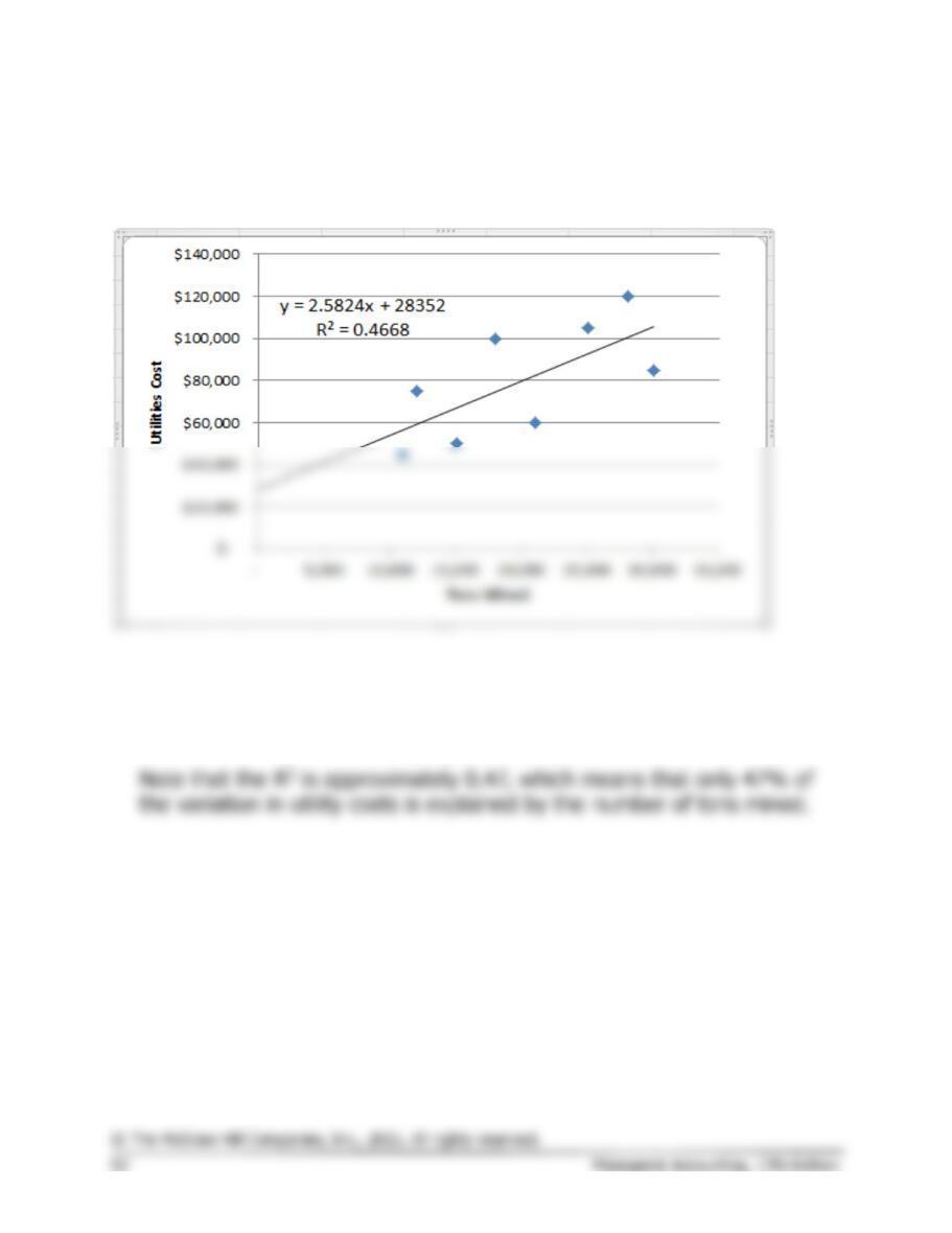
1. The scattergraph plot and regression estimates of fixed and variable
costs using Microsoft Excel are shown below:
The cost formula, in the form
Y
=
a
+
bX
, using tons mined as the
activity base is $28,352 per quarter plus $2.58 per ton mined, or
Y = $28,352 + $2.58X
Problem 5A-6 (continued)
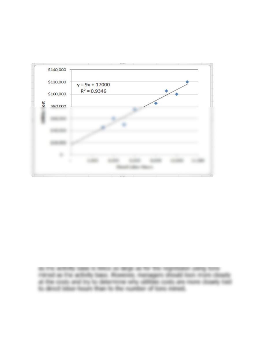
2. The scattergraph plot and regression estimates of fixed and variable
costs using Microsoft Excel are shown below:
The cost formula, in the form
Y
=
a
+
bX
, using direct labor-hours as
the activity base is $17,000 per quarter plus $9.00 per direct labor-hour,
or:
Y = $17,000 + $9.00X
Note that the R2 is approximately 0.93, which means that 93% of the
variation in utility costs is explained by direct labor-hours. This is a very
high R2 which is an indication of a very good fit.
3. The company should probably use direct labor-hours as the activity
base, since the fit of the regression line to the data is much tighter than
it is with tons mined. The R2 for the regression using direct labor-hours