5
Cost Estimation
Solutions to Review Questions
5-1.
5-2.
5-3.
Engineering estimates are particularly helpful when:
• Attempting to compare company operations with standards;
5-4.
The biggest problem likely to be encountered from the indiscriminate use of regression
methods is that the model may not have any logical foundation. This may result in a
5-5.
The longer the data series used in the analysis, the easier it is to see a trend in the data
when using the scattergraph method. When using any method, the longer the data
5-6.
5-7.
5-8.
5-9.
Three common implementation problems with regression analysis are nonlinear
5-10.
5-11.
Common data problems when estimating costs include missing data, outliers, allocated
Solutions to Critical Analysis and Discussion Questions
5-12.
a. Direct labor would be fixed if a union contract limited the company’s ability to lay off
5-13.
Account analysis incorporates the judgment of the executive where experience would
5-14.
Data in the historical accounting records should only be used insofar as they are likely
5-15.
One may:
5-16.
5-17.
It is possible for empirical data to show a negative intercept even though fixed costs
cannot be negative. It may be that the slope of the cost curve is particularly steep over
5-18.
5-19.
5-20.
5-21.
You should probably tell the executive about the error. If correcting the errors does not
5-22.
5-23.
Answers will vary. (1) Income tax preparers become more proficient as they learn; (2)
5-24.
5-25.
5-26.
Data from previous products, which are likely to be similar, provide information about
5-27.
It is certainly possible that for this example a statistical analysis is best. However, it
Solutions to Exercises
5-28. (15 min.) Methods of Estimating Costs―Engineering Estimates: Custom
Homebuilders.
Administrative costs ……………………………………
Building costs – per square foot (moderate) ….
(3,000 x $150 =)
Appliances (moderate) ………………………………..
Utilities costs (if required) …………………………….
5-29. (15 min.) Methods of Estimating Costs – Engineering Estimates: Twain
Services.
Guru cost (per hour) ……………………………………
(10 x $900 =)
$9,000
Helper cost (per hour) ………………………………….
25,000
Estimated consultant and miscellaneous cost …
G&A costs ………………………………………………….
57,525
5-30. (15 min.) Methods of Estimating Costs—Account Analysis: Portland
Products.
a. Cost estimate with new costs and volume.
Cost Item
Last Year’s
Cost
(1)
Cost
Change
(1 + Cost
Increase)
(2)
This Year’s
Cost
(at last
year’s
volume)
(1) x (2) =
(3)
Growth in
Volume
(4)
This Year’s
Cost
(3) x (4) = (5)
5-31. (15 min.) Methods of Estimating Costs—Account Analysis: Hal’s
Accounting Services.
a. Cost estimate with new costs and volume.
Cost Item
Year 1
Cost
(1)
Cost
Change
(1 + Cost
Increase)
(2)
Year 2 Cost
(at last
year’s
volume)
(1) x (2) =
(3)
Growth
in
Volume
(4)
Year 2 Cost
(3) x (4) = (5)
b. Costs per unit:
5-32. (10 min.) Methods of Estimating Costs—High-Low, Ethical Issues: Oak
Island Amusements Center.
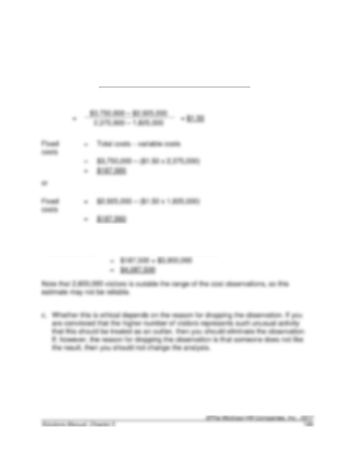
a.
Variable cost =
Cost at highest activity – cost at lowest activity
Highest activity – lowest activity
costs
=
$3,750,000 – ($1.50 x 2,375,000)
costs
b.
Maintenance costs
=
$187,500 + ($1.50 x 2,600,000)
=
5-33. (25 min.) Methods of Estimating Costs—High-Low: Adriana Corporation.
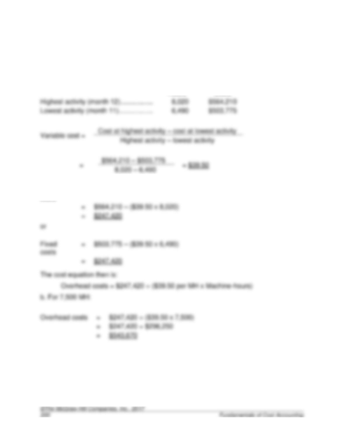
a. High-low estimate
Machine-
Hours
Overhead
Costs
Lowest activity (month 11) ………………
Fixed
costs
=
Total costs – variable costs
=
$564,210 – ($39.50 x 8,020)
Fixed
costs
=
$503,775 – ($39.50 x 6,490)
Overhead costs
=
$247,420 + ($39.50 x 7,500)
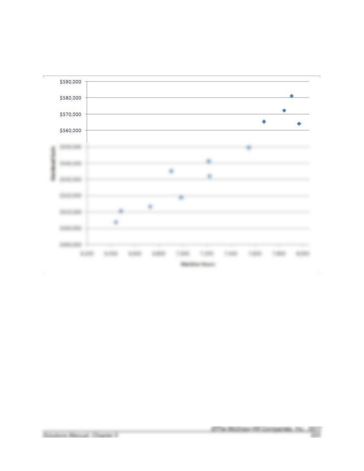
5-34. (15 min.) Methods of Estimating Costs—Scattergraph: Adriana Corporation.
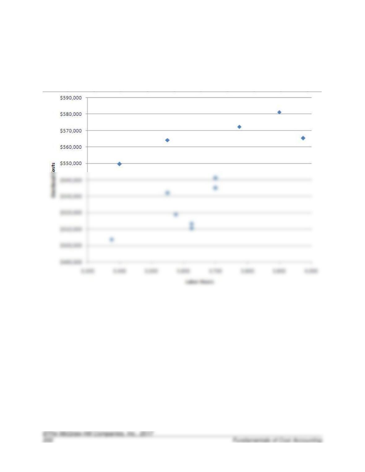
5-35. (15 min.) Methods of Estimating Costs—Scattergraph: Adriana
Corporation.
5-36. (10 min.) Methods of Estimating Costs—Simple Regression: Adriana
Corporation.
Simple regression estimate (note that the estimated 9,000 machine hours is outside the
relevant range):
5-37. (10 min.) Methods of Estimating Costs—Simple Regression: Adriana
Corporation.
Simple regression estimate (note that the estimated 3,000 machine hours is outside the
relevant range):
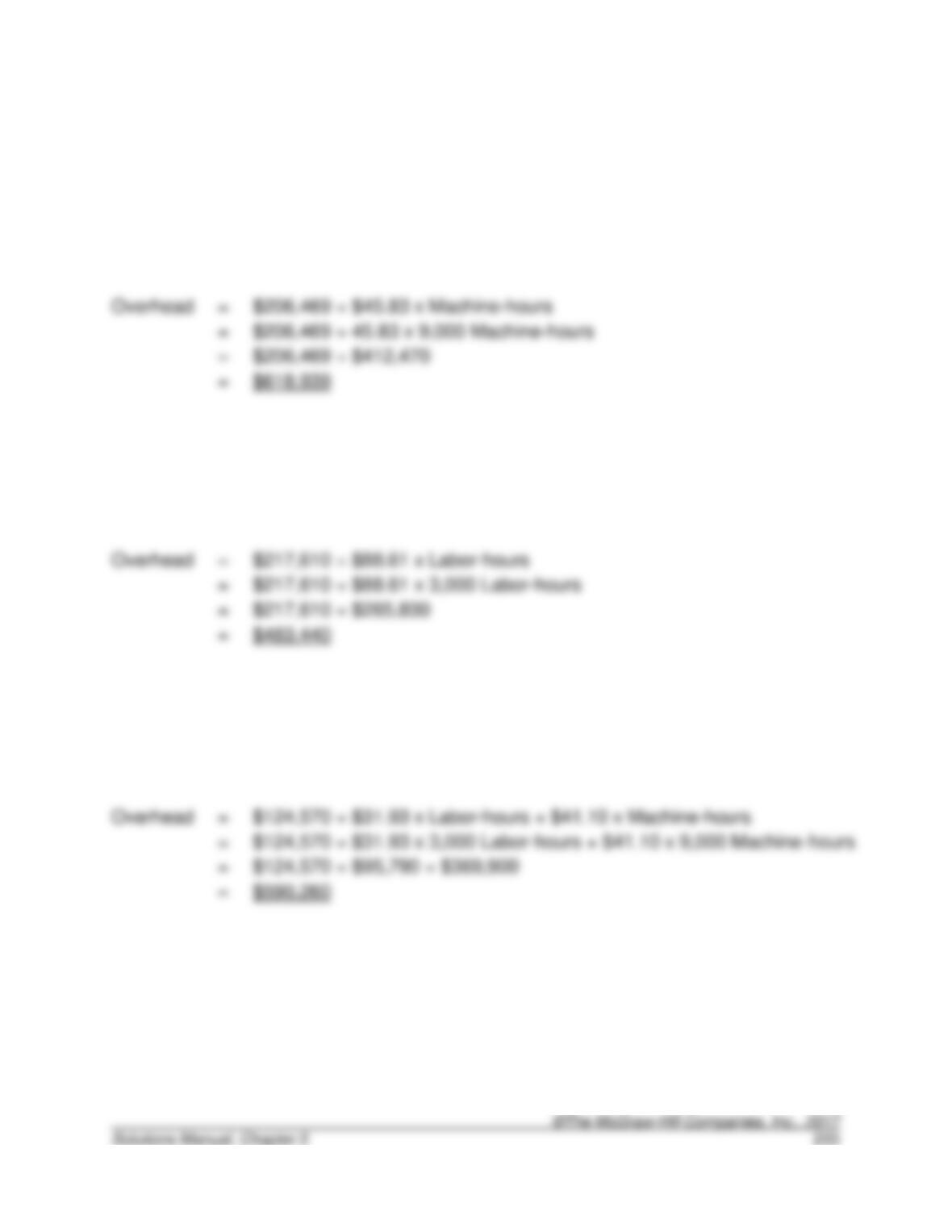
5-38. (20 min.) Methods of Estimating Costs—Multiple Regression: Adriana
Corporation.
Multiple regression estimate (note that the estimated 9,000 machine hours and 3,000
direct labor hours are outside the relevant range):
5-39. (40 min.) Methods of Estimating Costs—High-Low: Davis Stores.
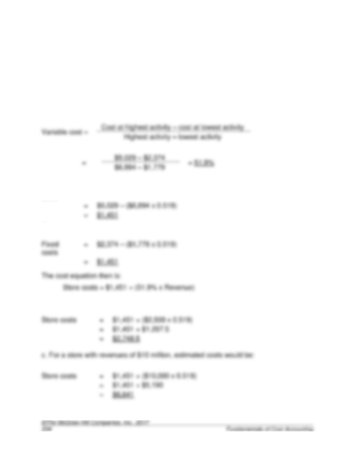
a. High-low estimate
Revenues
Costs
Highest activity (Store 107) …………….
$6,894
$5,029
Lowest activity (Store 108) ……………..
$1,779
$2,374
Fixed
costs
=
Total costs – variable costs
=
$5,029 – ($6,894 x 0.519)
or
Fixed
costs
=
$2,374 – ($1,779 x 0.519)
Store costs
=
$1,451 + ($2,500 x 0.519)
=
$1,451 + $1,297.5
Store costs
=
$1,451 + ($10,000 x 0.519)
=
$1,451 + $5,190
b. For a store with revenues of $2.5 million, estimated costs would be:
5-39 (continued)
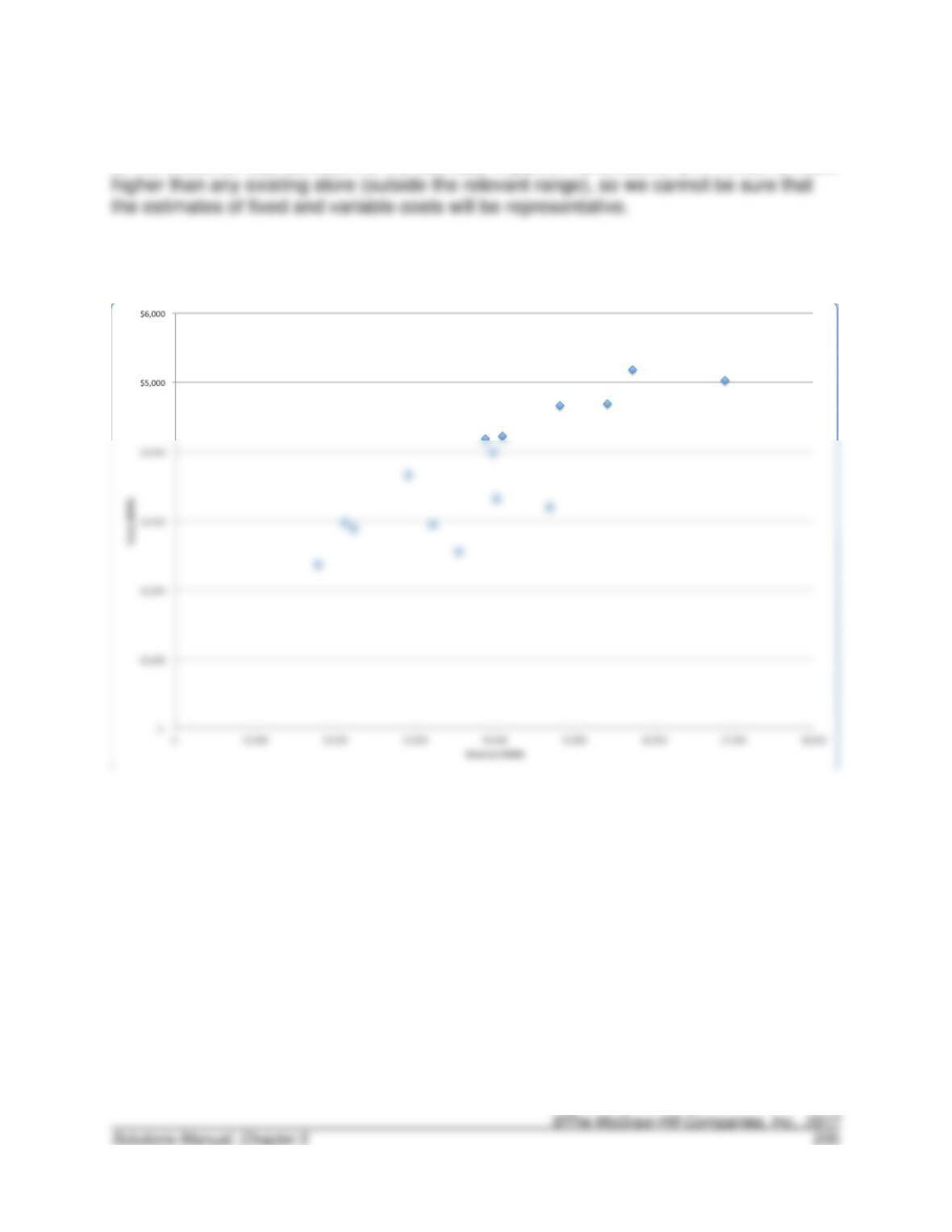
d. We would be less confident of the estimate in part c. Revenues of $10 million is much
5-40. (15 min.) Methods of Estimating Costs—Scattergraph: Davis Stores.
5-41. (10 min.) Methods of Estimating Costs—Simple Regression: Davis Stores.
a. Simple regression estimate (note that the estimated $2.5 million is inside the relevant
range):
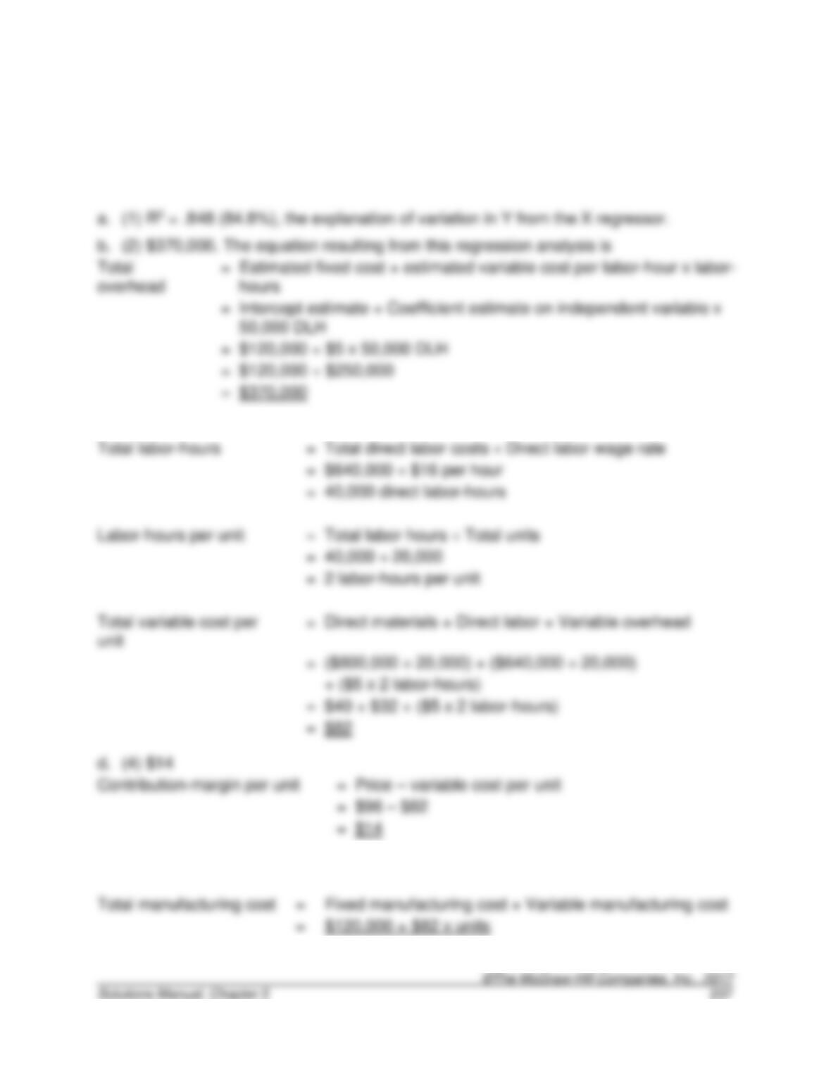
5-42. (20 min.) Interpretation of Regression Results—Multiple Choice: Cortez
Company.
c. (2) $82
e. (4) Some other equation:
*CMA adapted
5-43. (15 min.) Interpretation of Regression Results: Brodie Company.
This problem is frequently encountered when applying analytical techniques to certain
costs. Quite often the advertising expenditures result in sales being generated in the
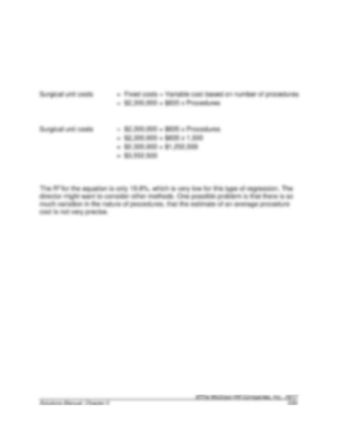
5-44. (15 min.) Interpretation of Regression Results: Ross Enterprises.
This problem is frequently encountered when applying analytical techniques to certain
5-45. (30 min.) Interpretation of Regression Results—Simple Regression.
a. Estimation equation for surgical unit costs:
b.
c.
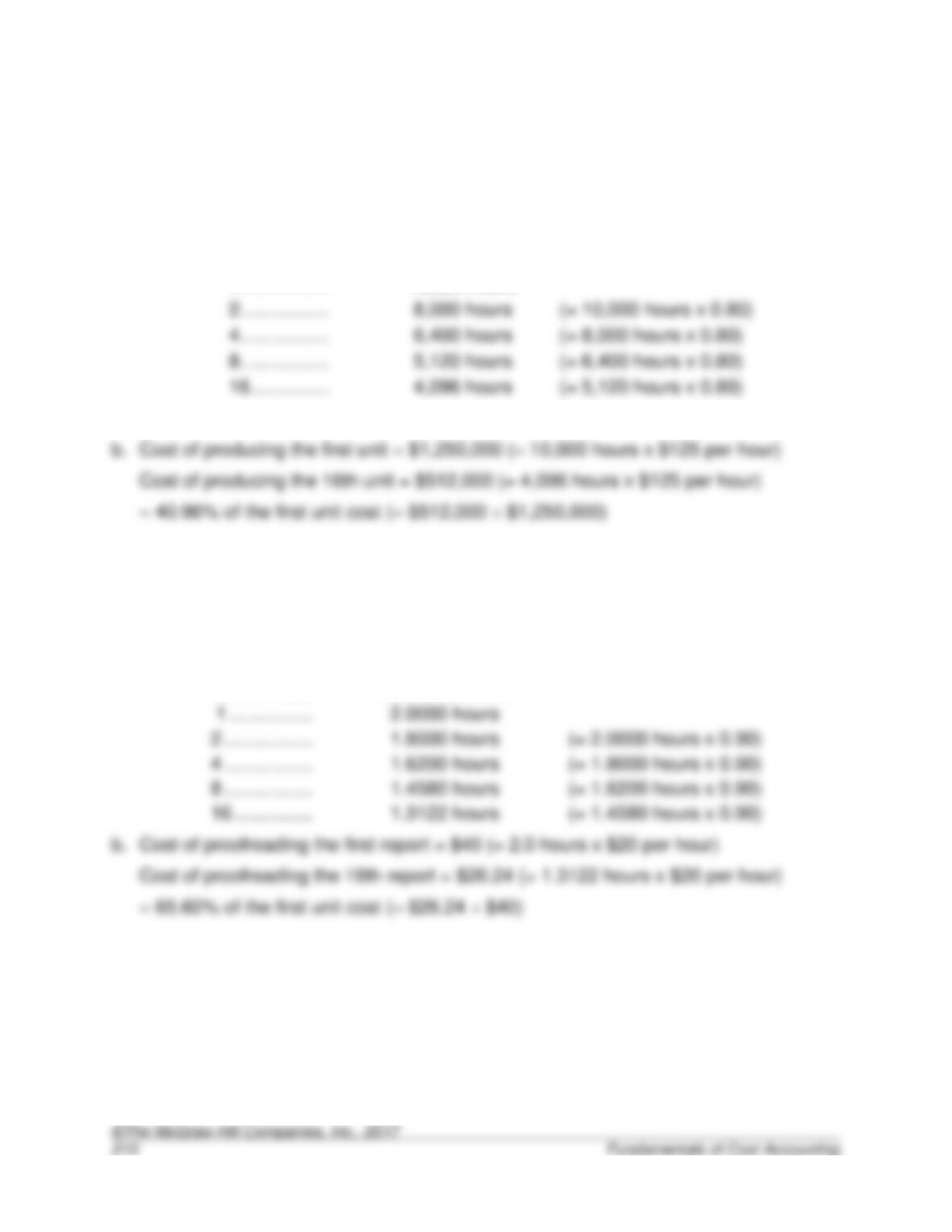
5-46. (20 min.) Learning Curves: General Dynamics.
a. The learning rate is 80% for every doubling of output:
Unit
Produced (X)
Time Required to
Produce the Xth Unit
1 ……………..
10,000 hours
2 ……………..
4 ……………..
5-47. (20 min.) Learning Curves: Whee, Cheatham, and Howe.
a. The learning rate is 90% for every doubling of output:
Financial
Statements
Proofread (X)
Time Required to
Proofread the Xth
Financial Statement
5-48. (20 min.) Learning Curves (Appendix B).
The formula for the time to produce unit z is Y =100 z–0.3219.
Substitute 5, 6, 7 for z, to obtain:
Unit (z)
Formula for Time to
Produce Unit z
Time to Produce Unit z
Solutions to Problems
5-49. (20 min.) Account Analysis.
a.
Activity
Total Cost
÷
Volume
=
Unit Cost
÷
3,650 accounts)
=
÷
30 analyses)
=
5-50. Regressions from Published Data.
5-51. Regressions from Published Data.
5-52. (30 min.) High-Low Method, Scattergraph: Cubicle Solutions.
a. High-low estimate
Support
Calls
Call Center
Cost
5-52 (continued)
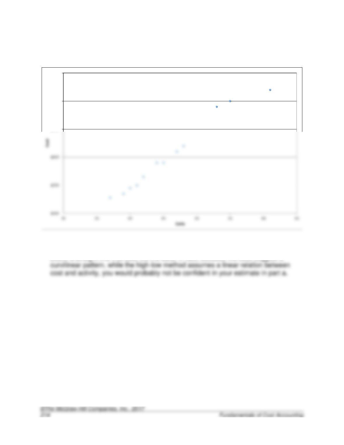
b. Scattergraph
$650
$700
$750
c. The scattergraph shows a reasonably linear pattern, but the high point would lie
below a straight line that best fits the data. In fact, because the data suggest a
5-53. (30 min.) High-Low Method, Scattergraph: Academy Products.
a. High-low estimate
Machine
Hours
Overhead
Costs
Highest activity (month 5) …………………….
1,035,000
$3,700,000
Lowest activity (month 1) ……………………..
630,000
660,000
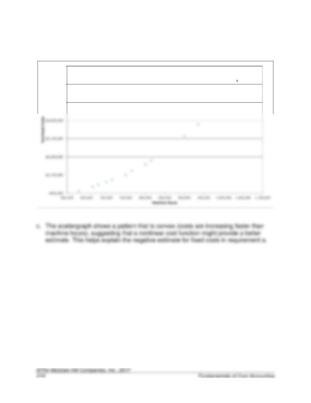
Fixed costs
=
Total costs – variable costs
5-53 (continued)
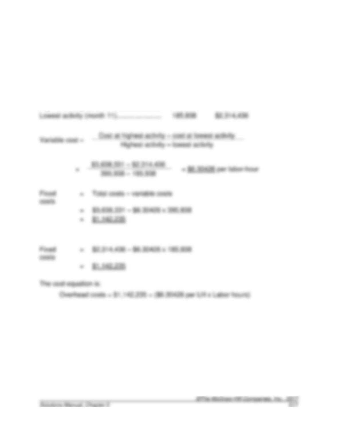
b. Scattergraph
$3,100,000
$3,600,000
$4,100,000
5-54. (40 min.) Interpretation of Regression Results—Simple Regression Using a
Spreadsheet: Lucas Plant.
a. High-low estimate
Labor
Hours
Overhead
Costs
Highest activity (month 16) …………………..
395,938
$3,638,331
or
5-54. (continued)
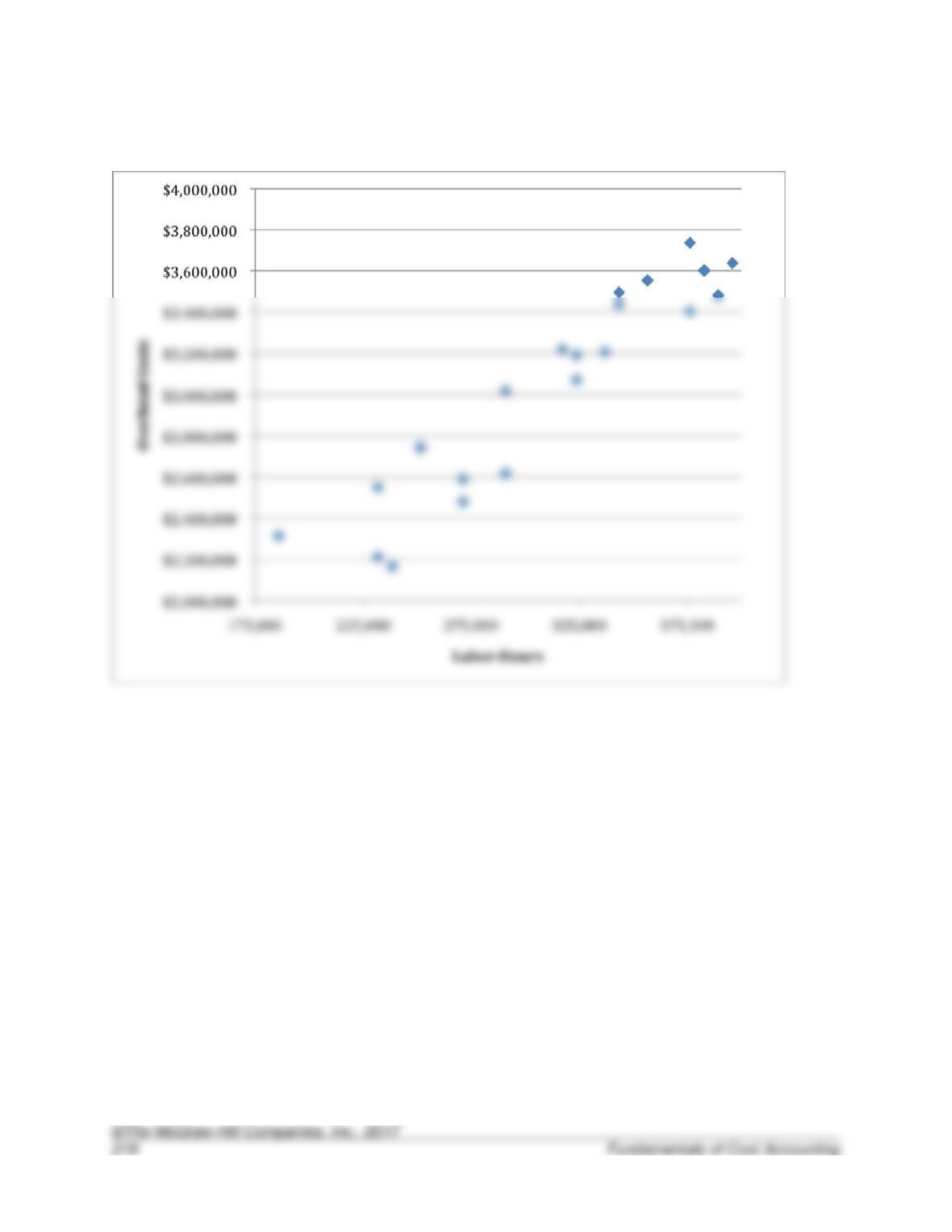
b. Scattergraph:
Note that two observations do not appear (separately) on this scattergraph. These are
observations 1 and 13. The dots actually overlap. These observations have the same
number of labor hours as observations 8 and 23, respectively, and the overhead costs
are close to the same.
5-54. (continued)
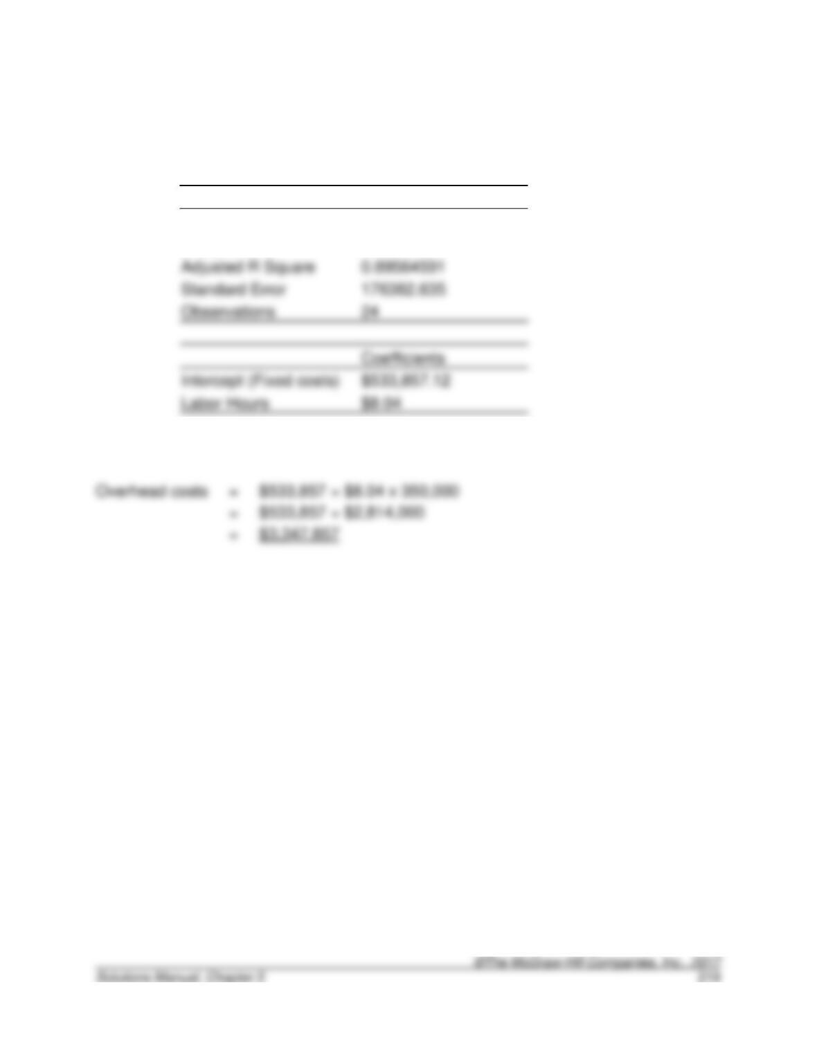
c. The results of the regression analysis are:
Regression Statistics
Multiple R
0.94877977
R Square
0.90018305
Adjusted R Square
0.89564591
Standard Error
176382.635
Observations
Coefficients
Intercept (Fixed costs)
Labor Hours
$8.04
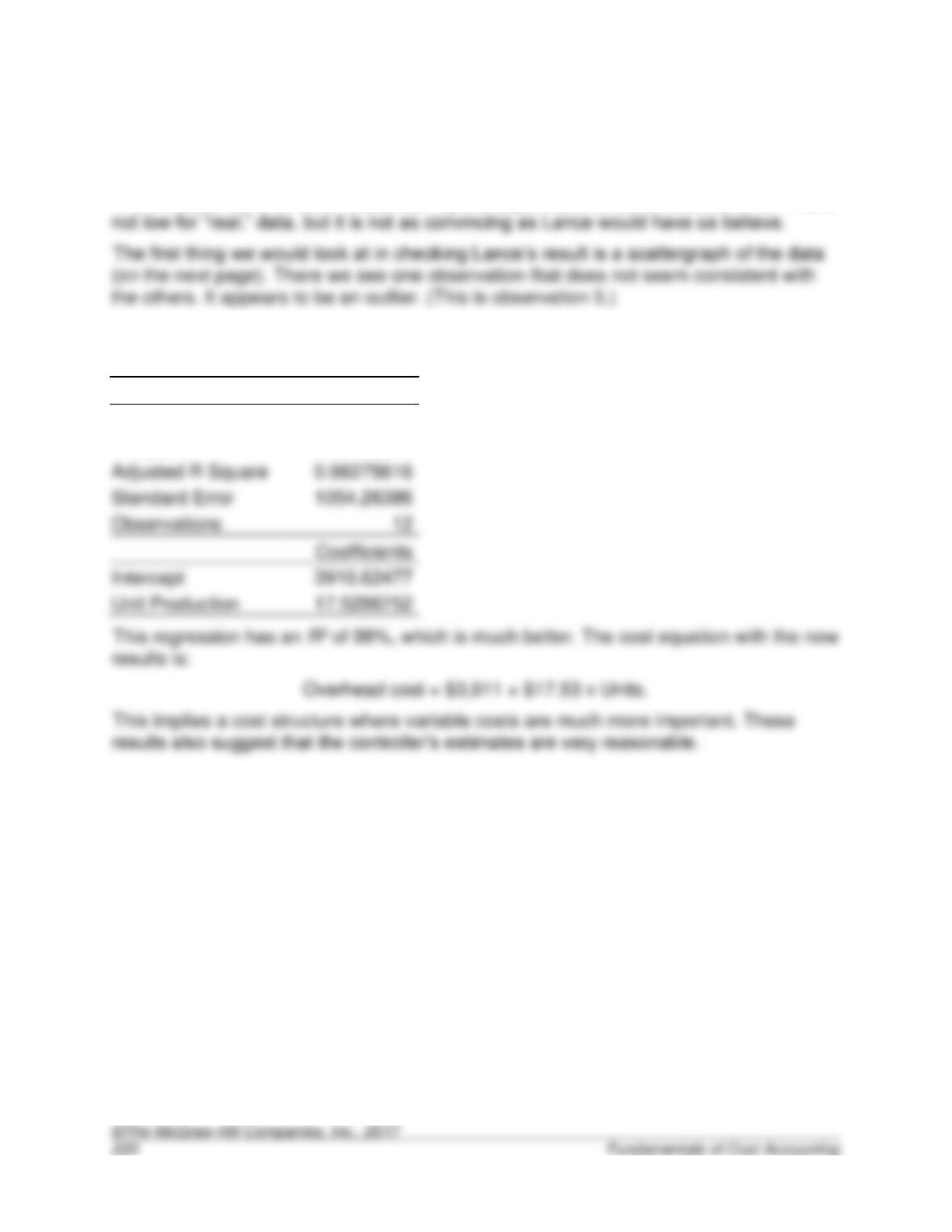
d.
5-55. (30 min.) Interpretation of Regression Results—Simple Regression..
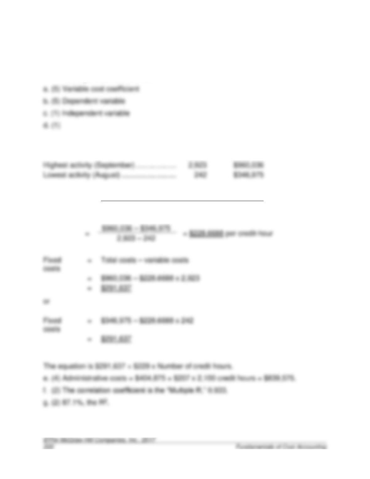
Although the correlation coefficient (or R) is 0.82, the R2, the percentage of the variation
in the independent variable “explained” by the dependent variable, is about 67%. This is
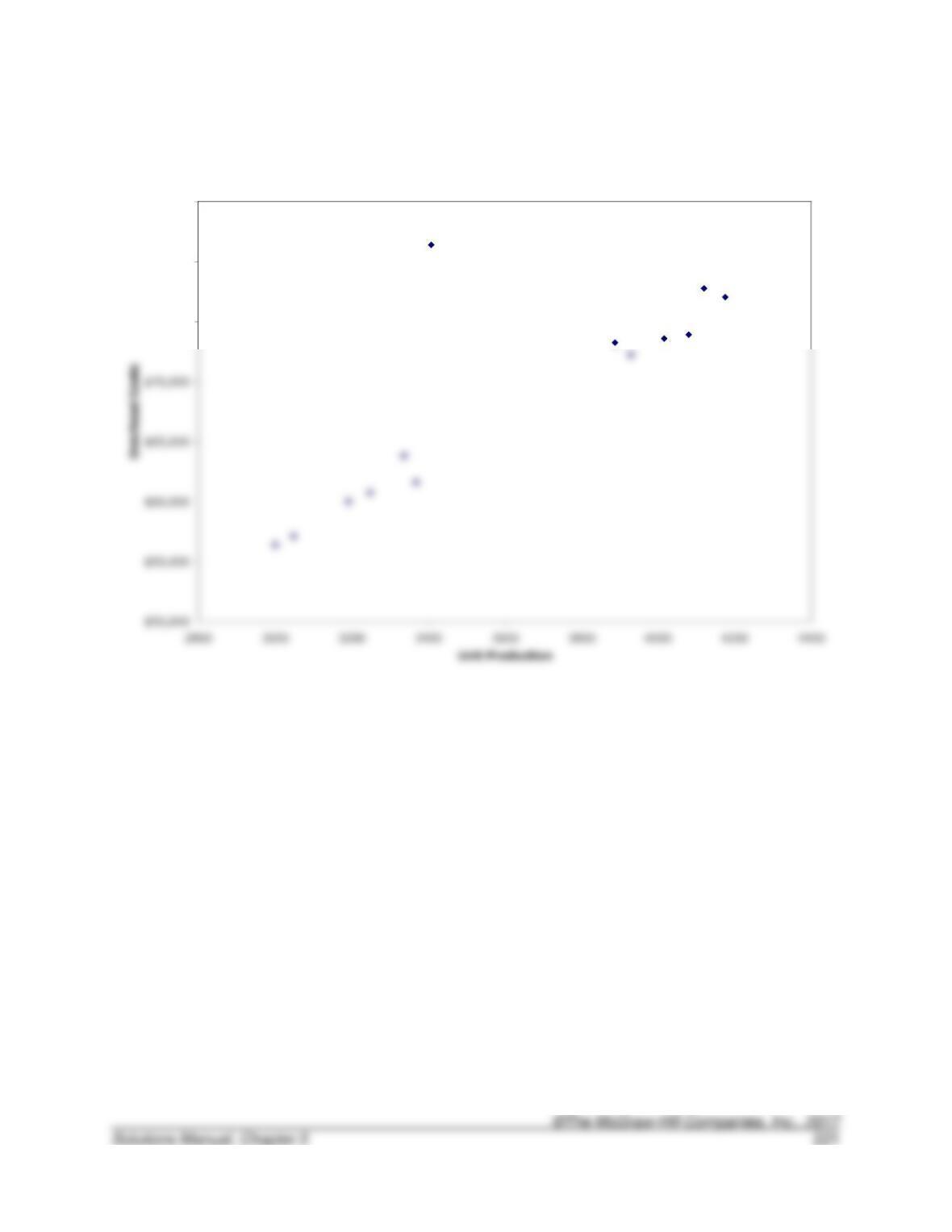
If the regression is re-estimated omitting observation 5, the results are:
Regression Statistics
Multiple R
0.99213093
R Square
0.98432378
Adjusted R Square
0.98275616
Standard Error
1054.26386
Observations
5-55. (continued)
$75,000
$80,000
$85,000
5-56. (30 Min.) Interpretation of Regression Results—Multiple Choice: Eastern
College Business School.
Credit-
hours
Administrative
Costs
Variable cost =
Cost at highest activity – cost at lowest activity
Highest activity – lowest activity
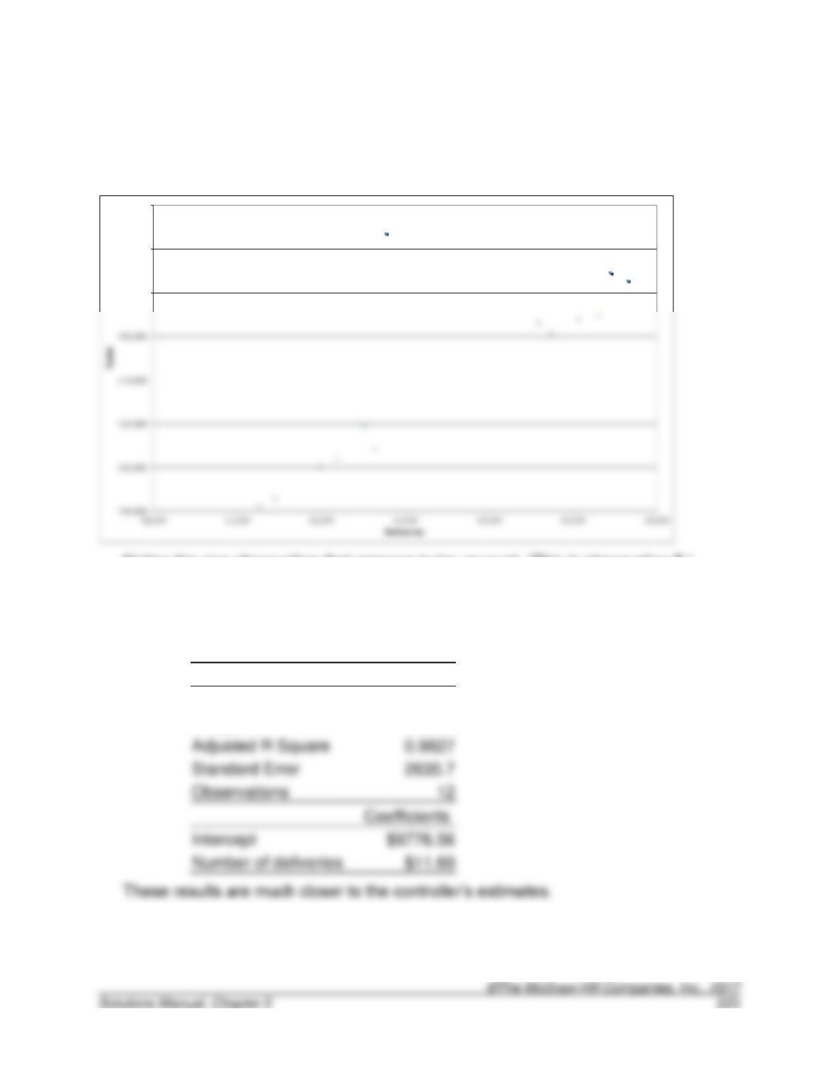
5-57. (30 Min.) Interpretation of Regression Results: Simple Regression.
a. The first step in understanding the difference is to prepare a scattergraph of the
data:
190,000
200,000
210,000
Notice the one observation that appears to be unusual. (This is observation 5.)
Without knowing more about the reasons for the high cost, we might want to treat it
as an “outlier” meaning we would estimate the regression without this observation.
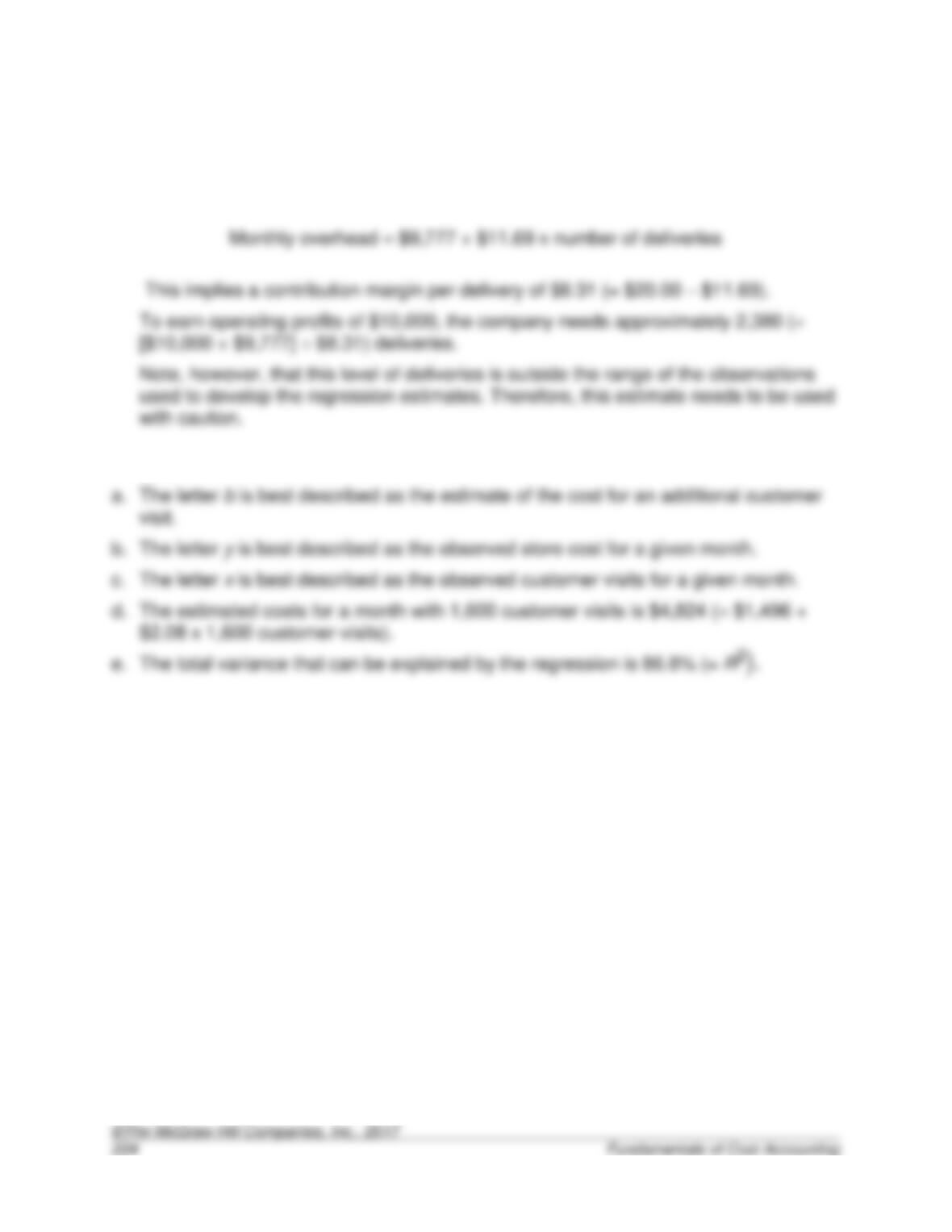
The results of that regression are:
Regression Statistics
Multiple R
0.9921
R Square
0.9843
Adjusted R Square
0.9827
Standard Error
2635.7
Observations
5-57 (continued)
b. Using the results from the “improved” regression, the cost equation for overhead
costs can be written as:
Monthly overhead = $9,777 + $11.69 x number of deliveries
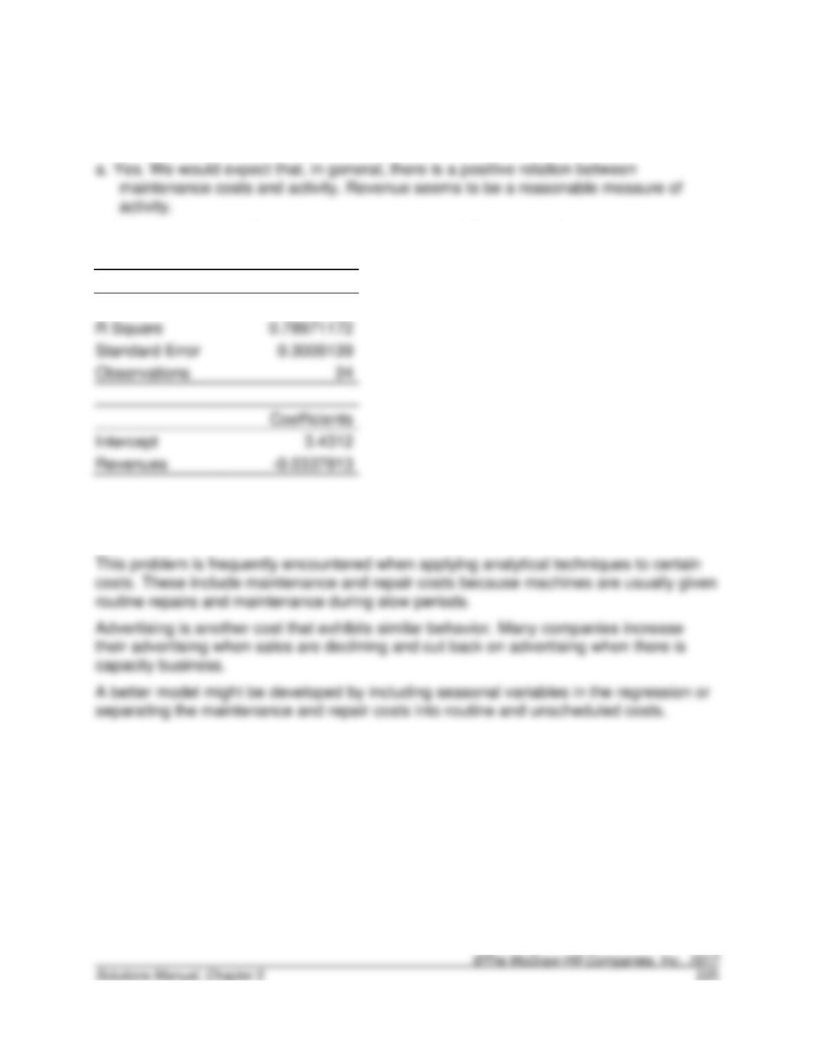
5-58. (30 Min.) Interpretation of Regression Results: Brews 4 U.
5-59. (30 Min.) Cost Estimation—Simple Regression: Arnie’s Arcade & Video
Palace.
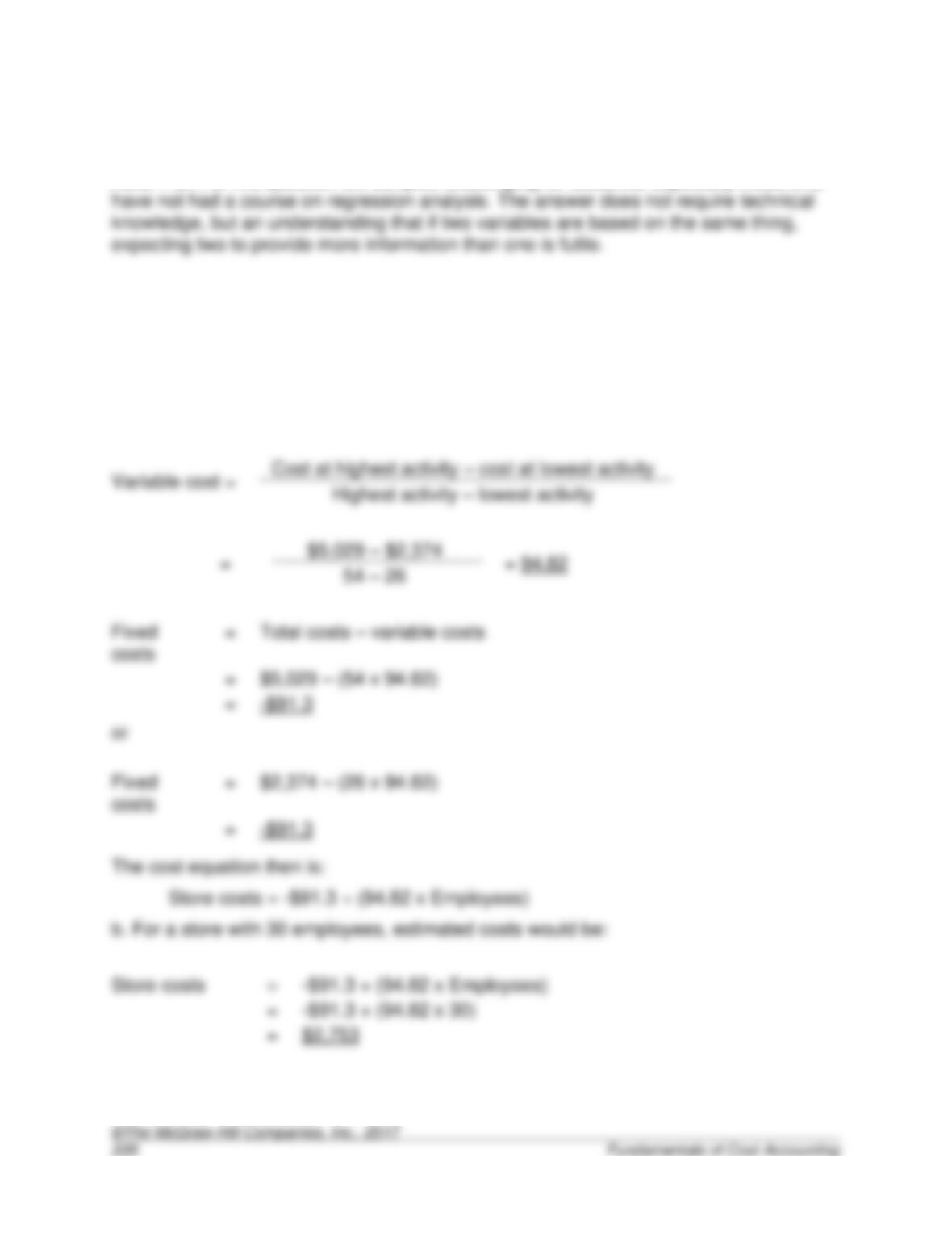
b. When we estimate the regression, we obtain the following results:
Regression Statistics
Multiple R
0.88865726
Standard Error
Observations
Intercept
Revenues
These suggest that maintenance costs are negatively related to revenues. The R2 is
reasonably high, suggesting a good fit.
5-60. (60 min.) Methods of Estimating Costs: Davis Stores.
Note: Part f of this question will be quite challenging for students, especially those who
a. High-low estimate
Employees
Costs
Highest activity (Store 107) …………….
54
$5,029
Lowest activity (Store 108) ……………..
26
$2,374
costs
=
$5,029 – (54 x 94.82)
costs
Store costs
=
-$91.3 + (94.82 x Employees)
=
-$91.3 + (94.82 x 30)
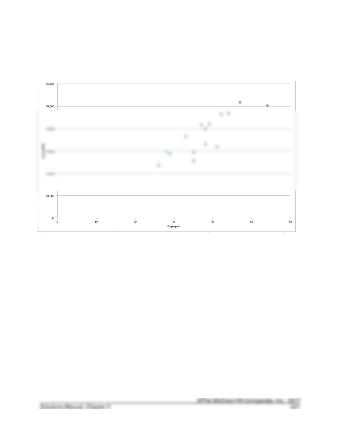
5-60 (continued)
c.
5-60 (continued)
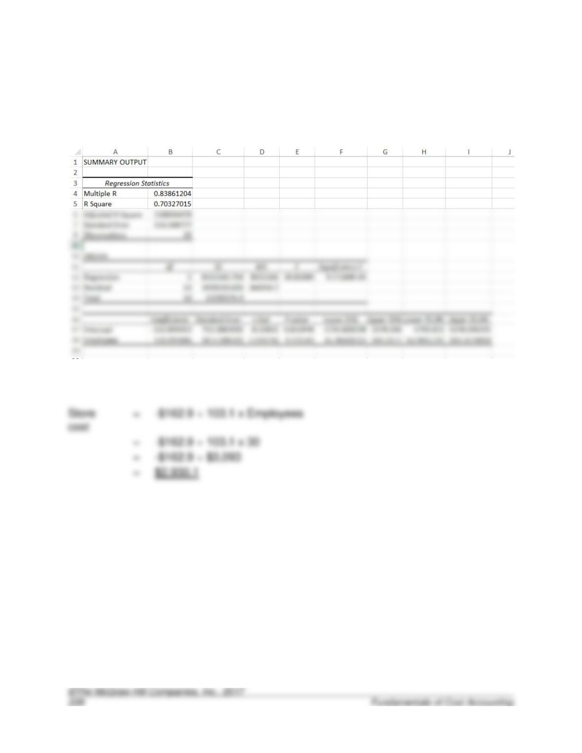
d. Simple regression estimates:
5-60 (continued)
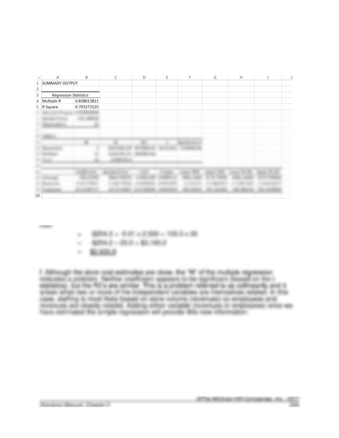
e. Multiple regression estimates:
cost
=
-$204.2 + -0.01 x 2,500 + 105.5 x 30
=
-$204.2 – 25.0 + $3,165.0
Store
=
-$204.2 + -0.01 x Revenues + 105.5 x Employees
5-61. (40 min.) Methods of Cost Analysis—Account Analysis, Simple and Multiple
Regression Using a Spreadsheet (Appendix A): Caiman Distribution
Partners.
a. Estimating equation based on account analysis:
Cost Item
Operating Cost
Fixed Cost
Variable
Supplies …………………………..
$ 350,000
$ 0
$ 350,000
Supervision ………………………
215,000
150,000
65,000
Truck expense ………………….
Building leases ………………….
855,000
550,000
305,000
Utilities …………………………….
215,000
125,000
90,000
Warehouse labor ……………….
Equipment leases ……………..
760,000
160,000
Data processing equipment ..
945,000
945,000
Other ……………………………….
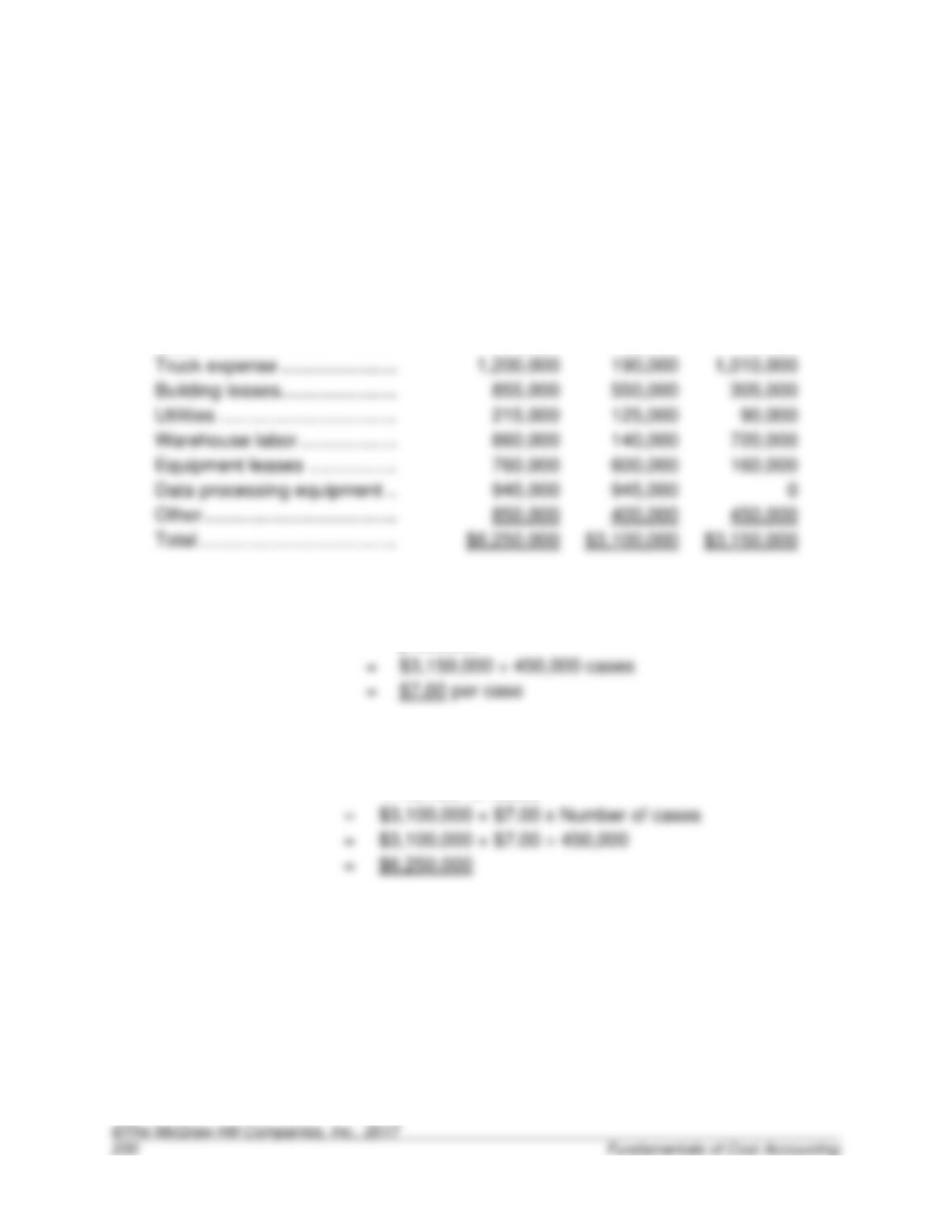
Variable cost per case
=
Total variable cost/Cases
produced
=
$3,150,000 ÷ 450,000 cases
Estimated overhead
=
Fixed overhead + Variable overhead per case
x Number of cases
=
$3,100,000 + $7.00 x Number of cases
=
5-61. (continued)
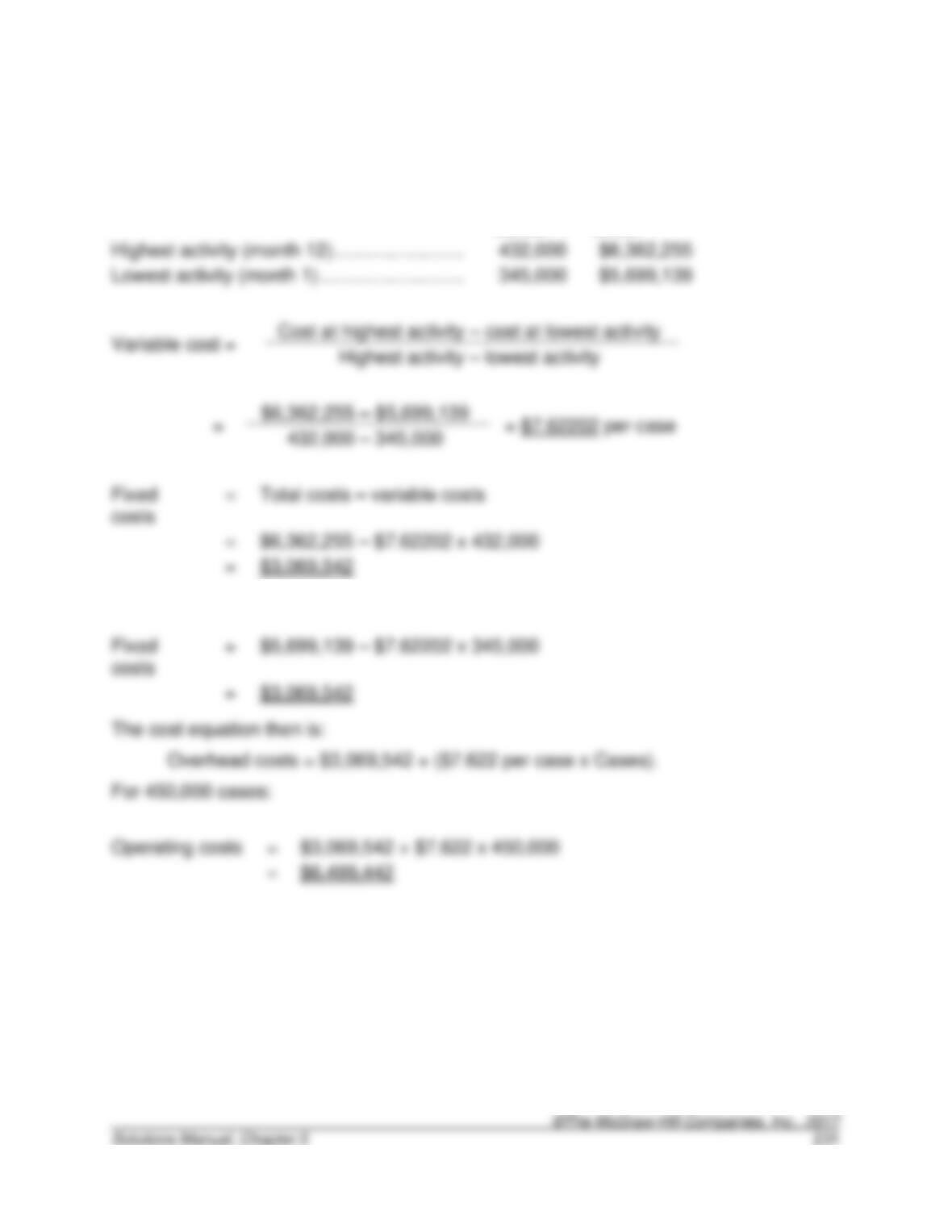
b. Cost estimate using high-low analysis.
Cases
Operating
Costs
Lowest activity (month 1) ……………………….
Fixed
costs
=
Total costs – variable costs
=
or
Fixed
costs
=
5-61. (continued)
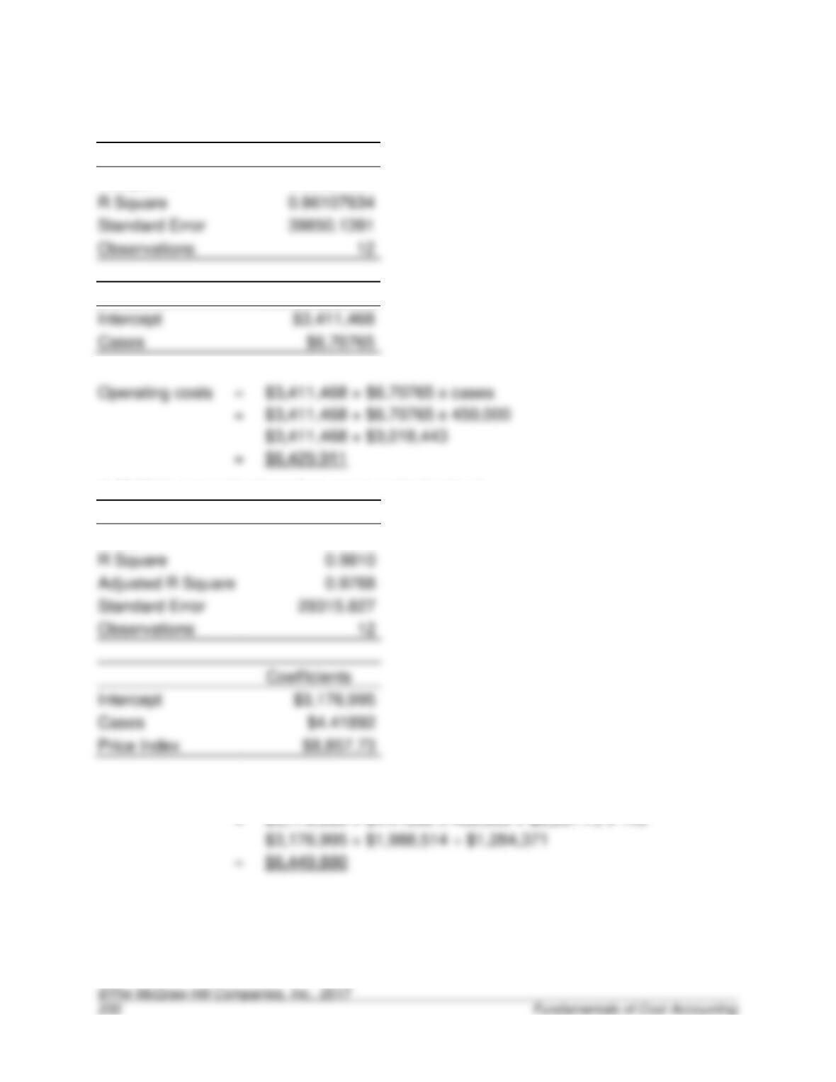
c. Simple regression based on cases:
Regression Statistics
Multiple R
0.98034501
R Square
0.96107634
Standard Error
39850.1391
Observations
Coefficients
Intercept
Cases
Operating costs
=
$3,411,468 + $6.70765 x cases
=
$3,411,468 + $6.70765 x 450,000
$3,411,468 + $3,018,443
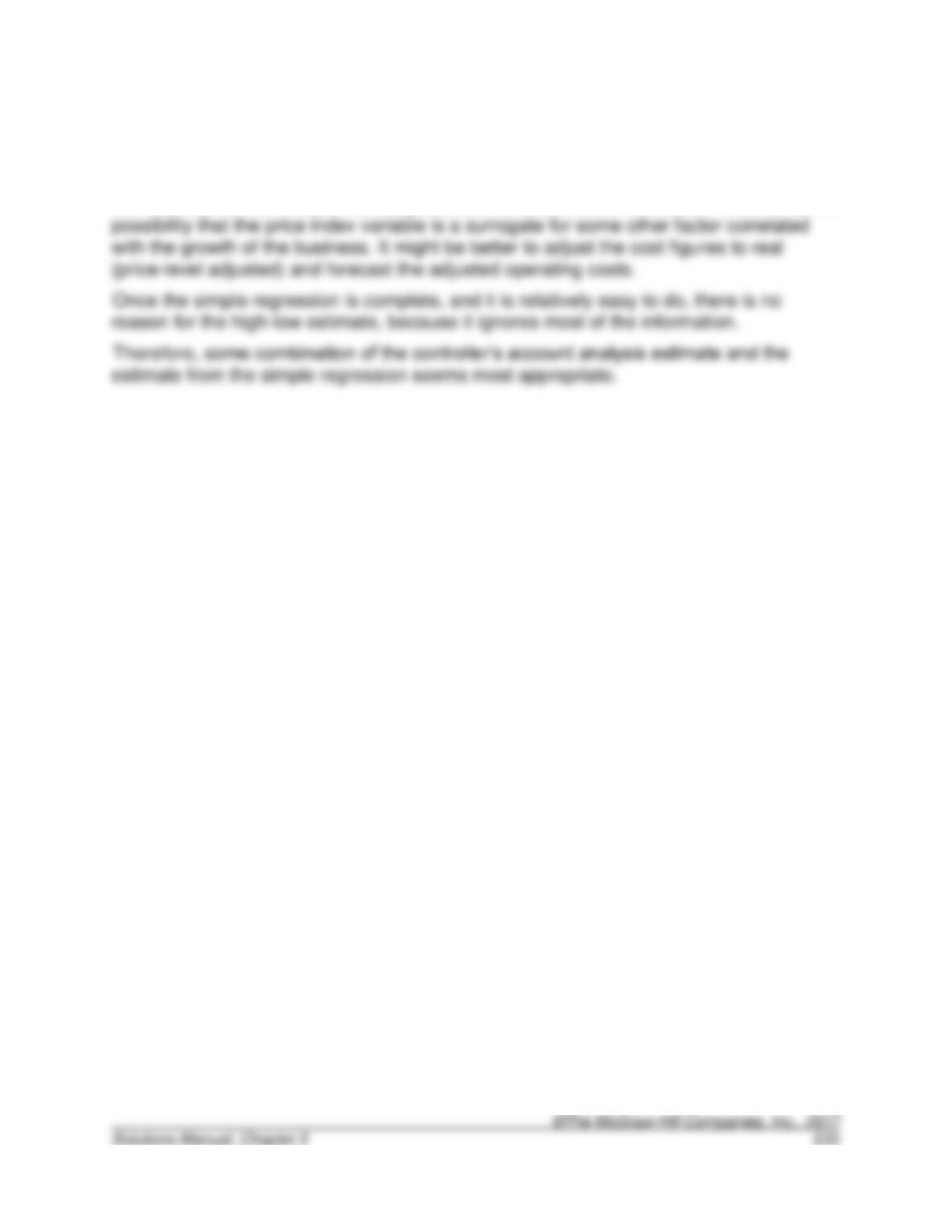
d. Multiple regression based on cases and price level.
Regression Statistics
Multiple R
0.9905
R Square
0.9810
Adjusted R Square
0.9768
Standard Error
Observations
Intercept
Cases
Price Index
Operating costs
=
$3,176,995 + $4.41892 x cases + $8,857.73 x Price level
=
$3,176,995 + $4.41892 x 450,000 + $8,857.73 x 145
$3,176,995 + $1,988,514 + $1,284,371
5-61. (continued)
e. Recommendation.
The multiple regression appears to improve the “fit” (compare the adjusted R2’s), but
the rationale for the inclusion of the price level as a cost driver is unclear. There is some
5-62. (40 min.) Learning Curves (Appendix 5B).
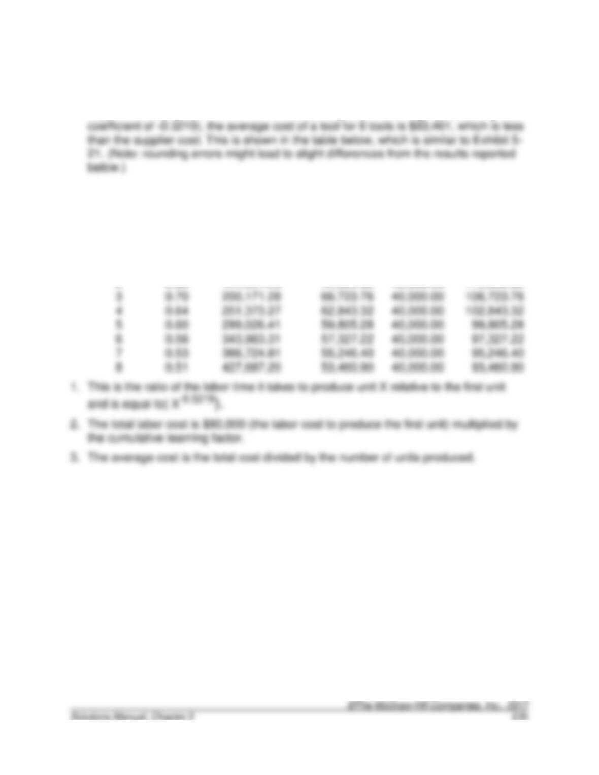
a. The learning rate coefficient is -0.152004, so the table in Exhibit 5-21 would be as
Labor Time
Required to
Produce the Xth
Unit (i.e, the Last
Cumulative
Unit
Single Unit
Total Time
Produced
Produced)1
in Labor
Total
Average Cost
(X)
(Y)
Hours2
Cost3
Per Unit4
1 ……………..
100.00
100
$5,000.00
$5,000.00
2 ……………..
3 ……………..
4 ……………..
5 ……………..
6 ……………..
7 ……………..
8 ……………..
5-63. (40 min.) Learning Curves (Appendix 5B): Krylon Company.
Krylon should produce the tool itself. With an 80 percent learning rate (learning rate
Unit
Learning
Total
Average
Total
Produced
Factor1
Labor
Labor Cost
Materials
Average
(X)
(Y)
Cost2
Per Unit3
Cost
Cost
1
1.00
$ 80,000.00
$80,000.00
$40,000.00
$120,000.00
2
0.80
144,001.25
72,000.62
40,000.00
112,000.62
3
0.70
200,171.28
66,723.76
40,000.00
106,723.76
4
0.64
251,373.27
62,843.32
40,000.00
102,843.32
5
0.60
299,026.41
59,805.28
40,000.00
6
0.56
343,963.31
57,327.22
40,000.00
7
0.53
386,724.81
55,246.40
40,000.00
8
0.51
427,687.20
53,460.90
40,000.00
Solutions to Integrative Cases
5-64. (60 min.) Cost Estimation, CVP Analysis, and Decision Making: Luke
Corporation.
This problem is more subtle than it might appear, because the student must consider
a. $2.24 per case.
This is a special order question similar to those discussed in Chapter 4. The relevant
cost is the variable production cost. (The problem states that no corporate overhead
will be allocated or affected by the order.) To determine the variable production cost,
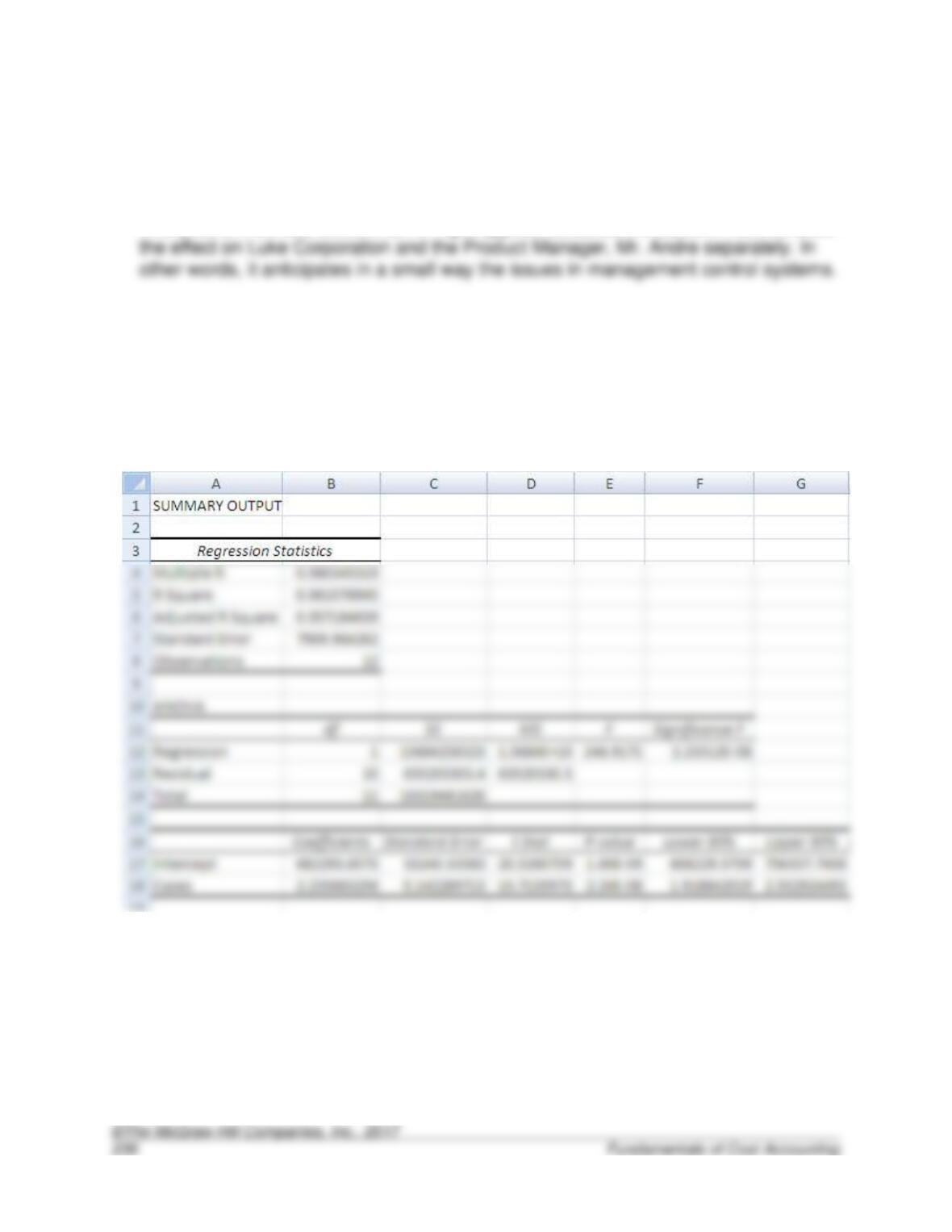
a regression analysis on the production data can be run. The results follow:
As shown, the estimated variable production cost is $2.24. This is the minumum that
can be charged without reducing profit.
5-64. (continued)
b. 242,120 cases.
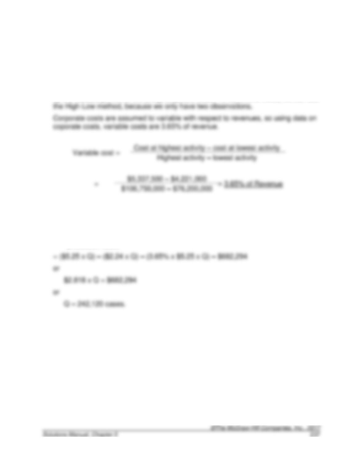
To break even on the product, Luke has to sell a sufficient number of cases to cover
fixed production costs on the product. The contribution margin, however, is lowered
by the variable portion of the (truly) corporate costs. To determine these, we can use
Let Q be the number of cases sold. Then, profit for Q cases is (note that the fixed
costs are from the analysis in part a):
Profit = Revenues – Variable product costs – Variable corporate costs – Fixed
production costs
5-64. (continued)
c. 274,565 cases.
This problem differs from requirement (c), because the the requirement that the
revenue from the product covers the production costs and the full 5% corporate cost
allocation makes the corporate cost allocation entirely variable. Therefore, the
number of cases to provide a profit equal to 5% of revenue (= 5% x $5.25 x Q) can
be determined as follows. Let Q be the number of cases sold. Then, profit for Q
cases is:
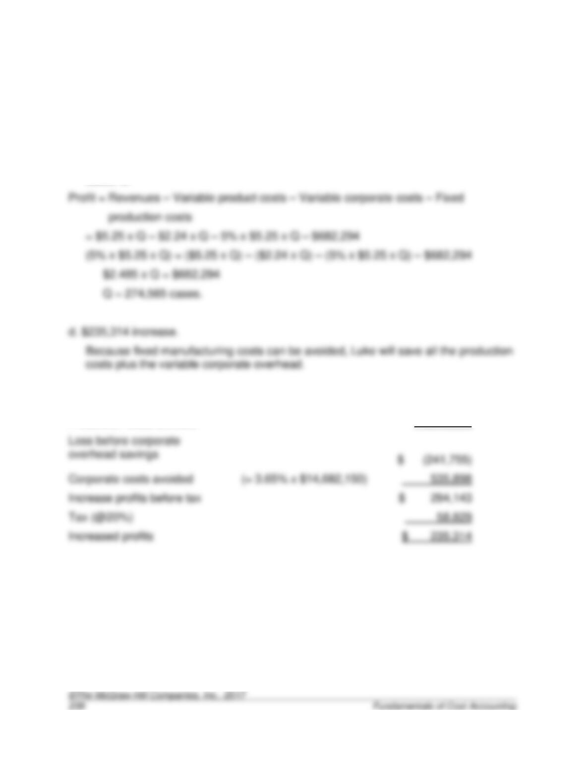
Lost revenue
$(14,682,150)
Production costs avoided
14,440,395
Corporate costs avoided
(= 3.65% x $14,682,150)
Increase profits before tax
Tax (@20%)