CHAPTER 5 Activity-Based Costing and Management
P 5-53 (Concluded)
4. This problem allows us to see what the accountin
g
cost per unit should
be b
y
providin
g
the abilit
y
to calculate the cost with and without the duffel
ba
g
s. With this perspective, it becomes eas
y
to see the benefits of the
accounting costs to each producing department, and this allocation probably
reflects quite well the consumption of accounting costs by each producing
department. The problem is the second-stage allocation. Direct labor hours
do not capture the consumption pattern of the individual products as they
pass through the departments. The distortion occurs, not in using transactions
to assign accounting costs to departments, but in using direct labor hours to
assign these costs to the two products.
CHAPTER 5 Activity-Based Costing and Management
P 5-54
1. Plantwide Rate = $990,000/440,000 DLHs = $2.25 per DLH
Overhead cost per unit:
Model A: ($2.25 × 140,000)/10,000 units = $31.50
Model B: ($2.25 × 300,000)/100,000 units = $6.75
Activit
y
rates:
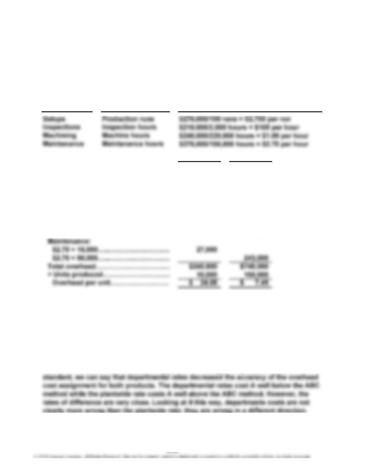
Driver
2. Overhead assignment: Model A Model B
Setups:
$2,700 × 40………………………………. $108,000
$2,700 × 60………………………………. $162,000
Inspections:
$105 × 800……………………………….. 84,000
$105 × 1,200……………………………
…
126,000
Machining:
$1.09 × 20,000…………………………… 21,800
$1.09 × 200,000…………………………
…
218,000
…
3. Departmental rates:
Overhead cost per unit:
Model A: ($3.50 × 10,000 machine hours) + ($0.90 × 130,000 direct labor hours)
/10,000 units = $15.20
Model B: ($3.50 × 170,000 machine hours) + ($0.90 × 270,000 direct labor hours)
/100,000 units = $8.38
4. A common justification is to use machine hours for machine-intensive departments
and labor hours for labor-intensive departments. Using activity-based costs as the
Activity Activity Rate
CHAPTER 5 Activity-Based Costing and Management
P 5-54
(
Concluded
)
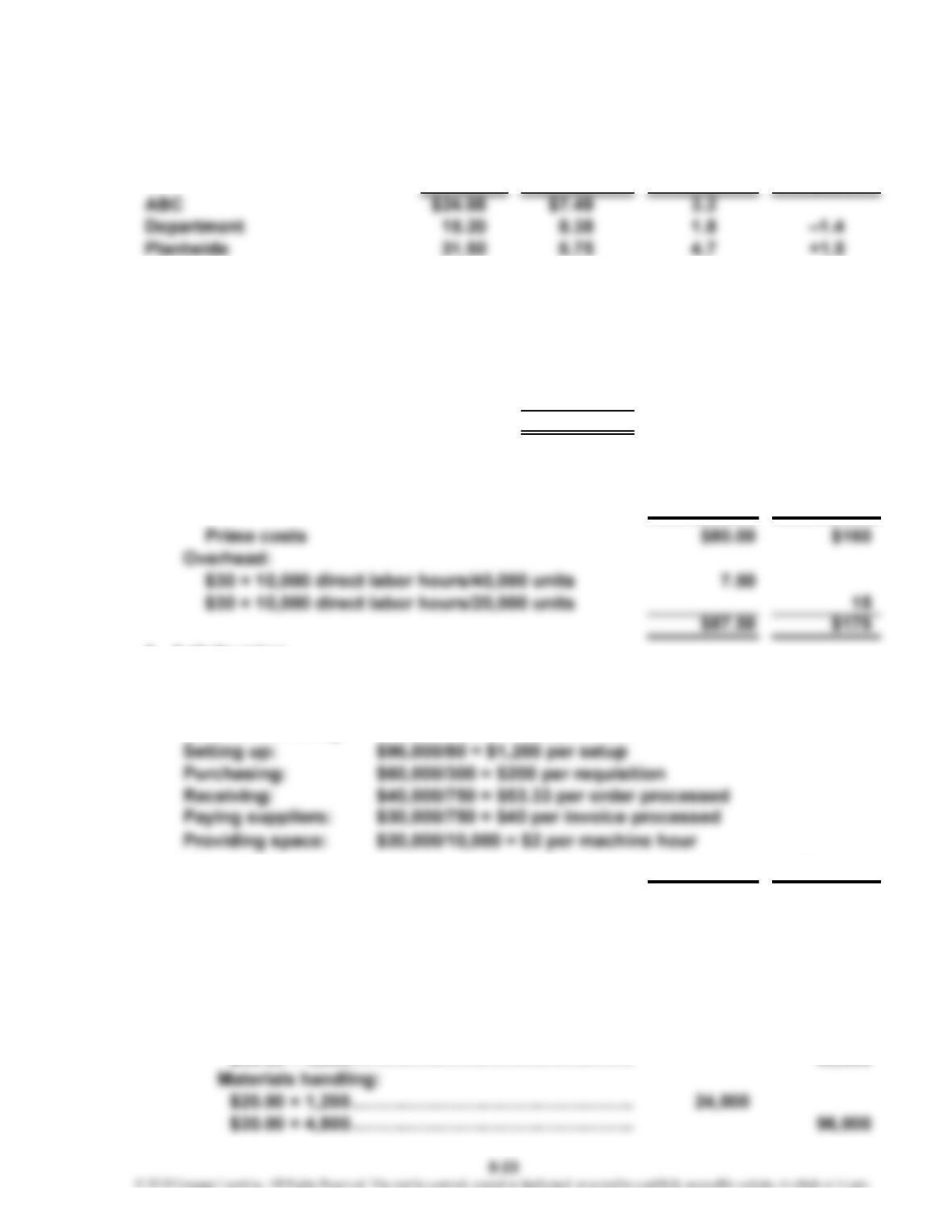
Costing by method:
A
B A/B Dif
f
P 5-55
1. Labor and gasoline are driver tracing.
Labor (0.75 × $120,000)…………………
…
$ 90,000 Time = Resource Driver
Gasoline ($3 × 6,000 moves)…………
…
18,000 Moves = Resource Driver
Depreciation (0.75 × $16,000)…………
…
12,000 Time = Resource Driver
Total cost……………………………… $120,000
2. Plantwide Rate = $600,000/20,000 direct labor hours
= $30 per DLH
Unit cost: Basic Deluxe
3. Activity rates:
Maintenance: $114,000/4,000 = $28.50 per maintenance hou
r
Engineering: $120,000/6,000 = $20 per engineering hou
r
Materials handling: $120,000/6,000 = $20 per move
Unit cost: Basic Deluxe
Prime costs ($80 × 40,000; $160 × 20,000)…………… $3,200,000 $3,200,000
Overhead:
Maintenance:
$28.50 × 1,000……….…………….…………………. 28,500
$28.50 × 3,000……….…………….…………………. 85,500
Engineering:
$20.00 × 1,500……….…………….…………………. 30,000
–
CHAPTER 5 Activity-Based Costing and Management
P 5-55
(
Continued
)
Setting up:
$1,200 × 16……….…………….………
…
19,200
$1,200 × 64……….…………….………
…
76,800
Paying suppliers:
$40 × 250……….…………….…………
…
10,000
$40 × 500……….…………….…………
…
20,000
Providing space:
$2 × 5,000……….…………….…………
…
10,000
$2 × 5,000……….…………….…………
…
10,000
…
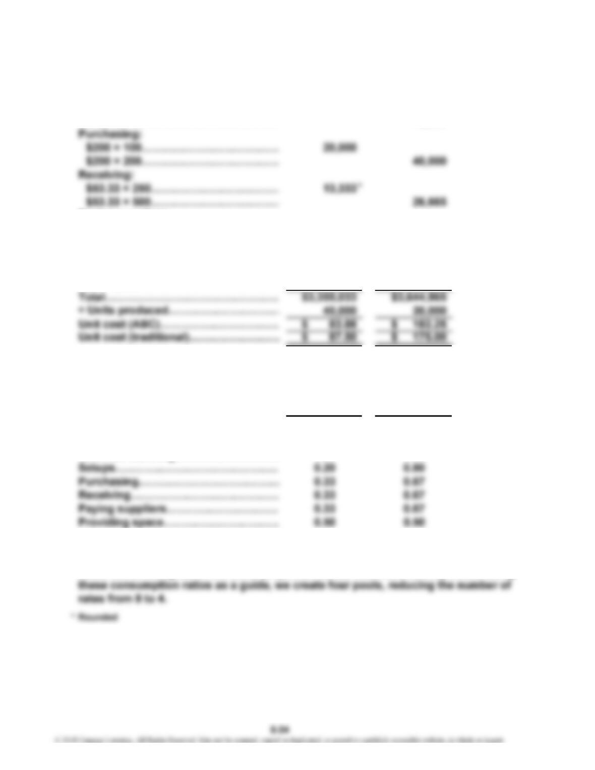
The ABC costs are more accurate (better tracing—closer representation of actual
resource consumption). This shows that the basic model was overcosted and the
deluxe model undercosted when the plantwide overhead rate was used.
4. Consumption ratios: Basic Deluxe
Maintenance……………….…………….
…
0.25 0.75
Engineering………………….……………
.
0.25 0.75
Materials handling………….……………
.
0.20 0.80
5. When products consume activities in the same proportion, the activities with the
same proportions can be combined into one pool. This is so because the pooled
costs will be assigned in the same proportion as the individual activity costs. Using
CHAPTER 5 Activity-Based Costing and Management
P 5-55
(
Concluded
)
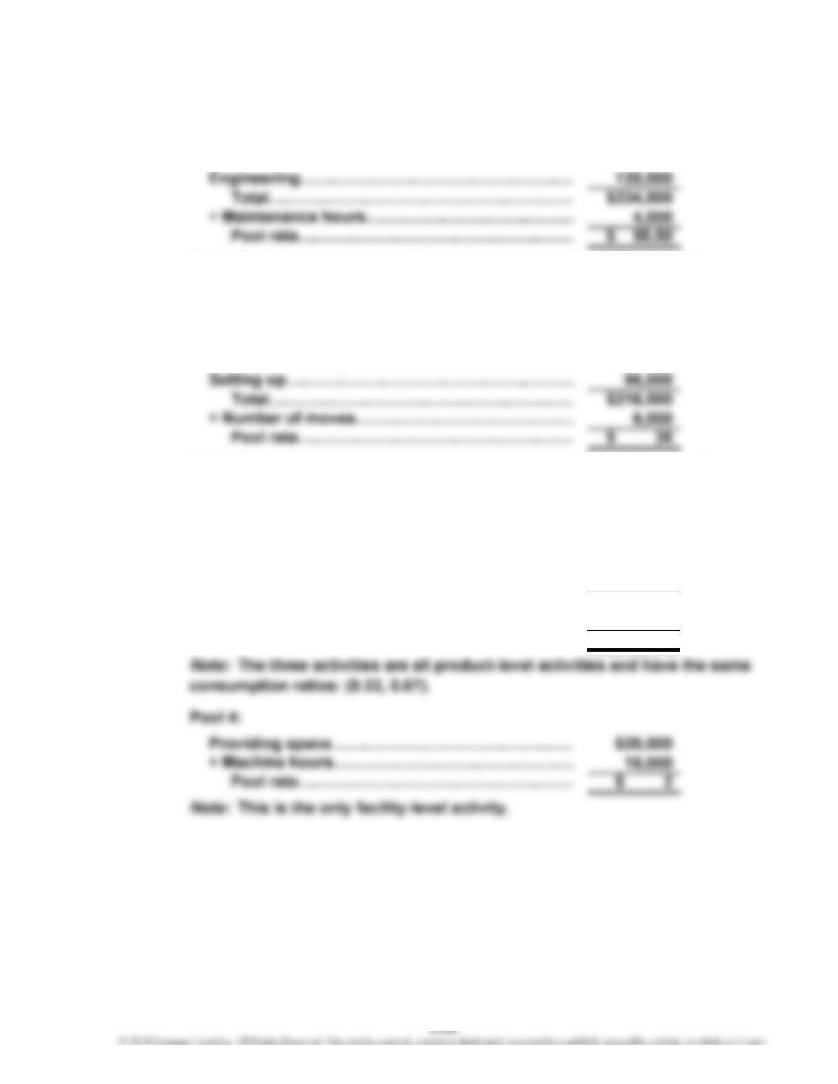
Pool 1:
Maintenance…………………………………………… $114,000
Note: Engineering hours could also be used as a driver. The activities are
grouped together because they have the same consumption ratios:
(0.25, 0.75).
Pool 2:
Materials handling……………………………………
…
$120,000
…
…
Note: Materials handling and setups have the same consumption ratios:
(0.20, 0.80). The number of setups could also be used as the pool driver.
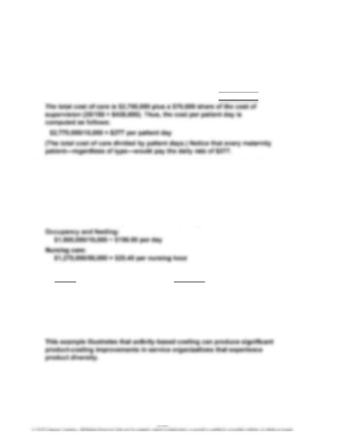
Pool 3:
Purchasing……………………………………………
…
$ 60,000
Receiving………………………………………………
…
40,000
Paying suppliers………………………………………
…
30,000
Total…………………………………………………
…
$130,000
÷ Orders processed…………………………………
…
750
Pool rate……………………………………………
…
$ 173.33
…
…
…
…
…
CHAPTER 5 Activity-Based Costing and Management
P 5-56
1. The cost of supervision is computed as follows:
Salary of supervisor (direct)………………………………… $ 80,000
Salary of secretary (direct)…………………………………
…
35,000
Other costs (direct)…………………………………………… 170,000
Assistants (3 × 0.75 × $60,000)……………………………
…
135,000
Total…………………………………………………………
…
$420,000
2. First, the cost of the secondary activity (supervision) must be assigned to
the primary activities (various nursing care activities) that consume it
(the driver is the number of nurses):
Maternity nursing care assignment:
25/150 × $420,000 = $70,000
Thus, the total cost of nursing care is $1,200,000 + $70,000 = $1,270,000.
Next, calculate the activity rates for the two primary activities:
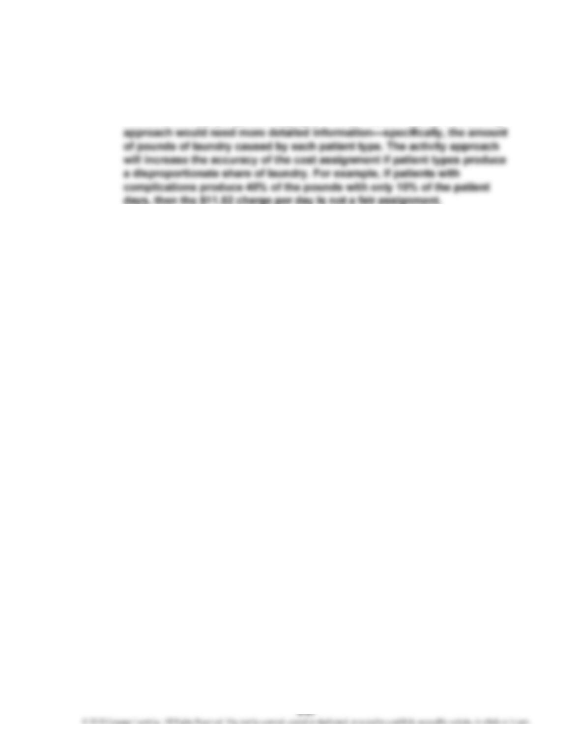
Finally, the cost per patient day type can be computed:
Patient Daily Rate
Normal…………………………………
…
$213.50
Cesarean………………………………
…
$308.75
Complications………………………… $658.00
a($150 × 7,000) + ($25.40 × 17,500)/7,000
b
($150 × 2,000) + ($25.40 × 12,500)/2,000
c($150 × 1,000) + ($25.40 × 20,000)/1,000
a
b
c
CHAPTER 5 Activity-Based Costing and Management
P 5-56
(
Concluded
)
3. The laundry department cost would increase the total cost of the maternity
department by $115,200 (240,000/1,250,000 × $600,000). This would
increase the cost per patient day by $11.52 ($115,200/10,000). The activity
CHAPTER 5 Activity-Based Costing and Management
P 5-57
1. Cost per Account = $6,105,000/75,000 accounts = $81.40
Average Fee per Month = $81.40/12 months = $6.78
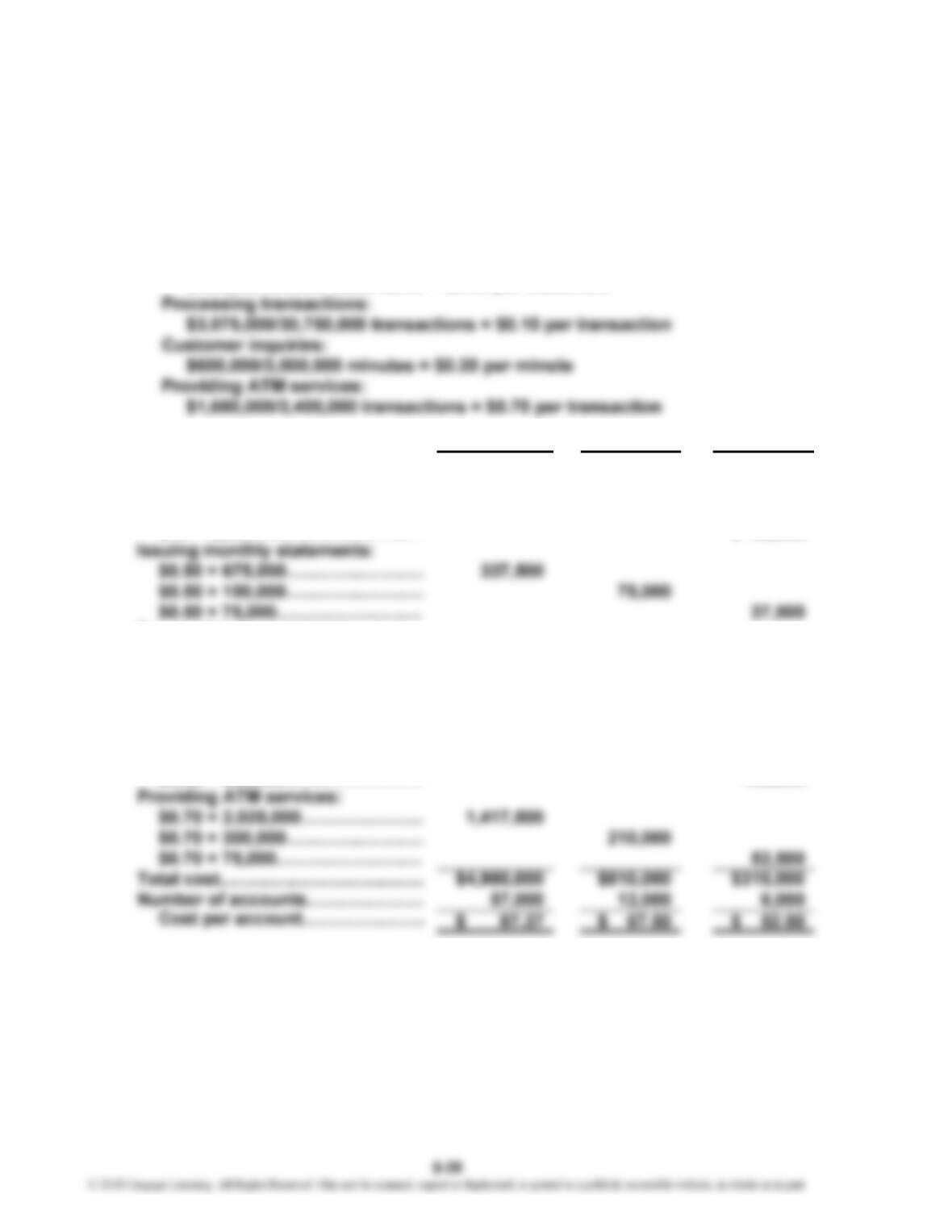
2. Activity rates:
Opening and closing accounts:
$300,000/30,000 accounts = $10 per account
Issuing monthly statements:
$
450,000/900,000 statements =
$
0.50 per statement
Costs assigned: Low Medium High
Opening and closing:
$10 × 22,500………………………
…
$ 225,000
$10 × 4,500………………………
…
$ 45,000
$10 × 3,000………………………
…
$ 30,000
…
…
Processing transactions:
$0.10 × 27,000,000………………
…
2,700,000
$0.10 × 3,000,000………………… 300,000
$0.10 × 750,000…………………
…
75,000
Customer inquiries:
$0.20 × 1,500,000………………… 300,000
$0.20 × 900,000…………………
…
180,000
…
…
CHAPTER 5 Activity-Based Costing and Management
P 5-57 (Concluded)
3. Average profit per account: $90.00 – $81.40 = $8.60
ABC profit measure:
Low-balance customers………………
…
$80.00 – $87.37 = $(7.37)
Medium-balance customers…………… $100.00 – $67.50 = $32.50
High-balance customers………………
…
$165.00 – $52.50 = $112.50
P 5-58
1. GAAP mandates that all nonmanufacturing costs be expensed during the
period in which they are incurred. GAAP is the most likely cause of the practice.
The limitations of GAAP-produced information for cost management should be
emphasized.
CHAPTER 5 Activity-Based Costing and Management
P 5-58
(
Continued
)
2. The average order-filling cost per unit produced is computed as follows:
$9,000,000/180,000,000* units = $0.05 per unit
*(600 × 100,000) + (1,000 × 60,000) + (1,500 × 40,000) = 180,000,000
Thus, order-filling costs are about 6 to 10% of the selling price, clearly not a
trivial amount.
Furthermore, the per-unit cost for individual product families can be computed
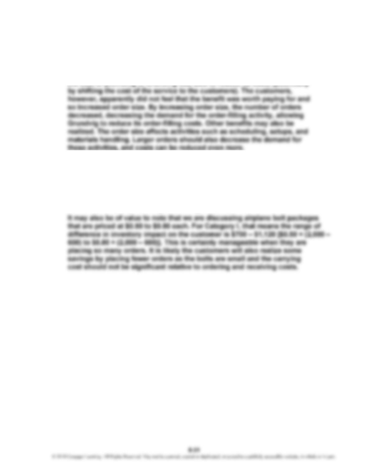
using the number of orders as the activity driver:
3. With the pricing incentive feature, the average order size has been increased
to 2,000 units for all three product families. The number of orders now
processed can be calculated as follows:
Orders = [(600 × 100,000) + (1,000 × 60,000) + (1,500 × 40,000)]/2,000
= 90,000
CHAPTER 5 Activity-Based Costing and Management
P 5-58 (Concluded)
Customers were placing smaller and more frequent orders than necessary.
They were receiving a benefit without being charged for it. By charging for
the benefit and allowing customers to decide whether the benefit is worth
Competitive advantage is created by providing the same customer value
for less cost or better value for the same or less cost. By reducing the
cost, Grundvig can increase customer value by providing a lower price
(decreasing customer sacrifice) or by providing some extra product
features without increasing the price (increasing customer realization,
holding customer sacrifice constant). This is made possible by the
decreased cost of producing and selling the bolts.
CHAPTER 5 Activity-Based Costing and Management
P 5-59
1. Supplier cost:
First, calculate the activity rates for assigning costs to suppliers:
Replacing engines:
Next, calculate the cost per engine by supplier:
Supplier cost:
Watson Johnson
Purchase cost:
$900 × 18,000………………………….…
…
$16,200,000
…
.
Repairing engines:
$720 × 2,440………………………………
…
1,756,800
$720 × 60………………………………..…
…
43,200
Total supplier cost…………………………
…
$19,738,800 $4,061,200
÷ Units supplied……………………….……
…
18,000 4,000
Unit cost…………………………………
…
$ 1,096.60 $ 1,015.30
The Johnson engine costs less when the full supplier effects are considered.
This is a better assessment of cost because it considers the costs that are
caused by the supplier due to poor quality, poor reliability, and poor delivery
performance.
CHAPTER 5 Activity-Based Costing and Management
P 5-60
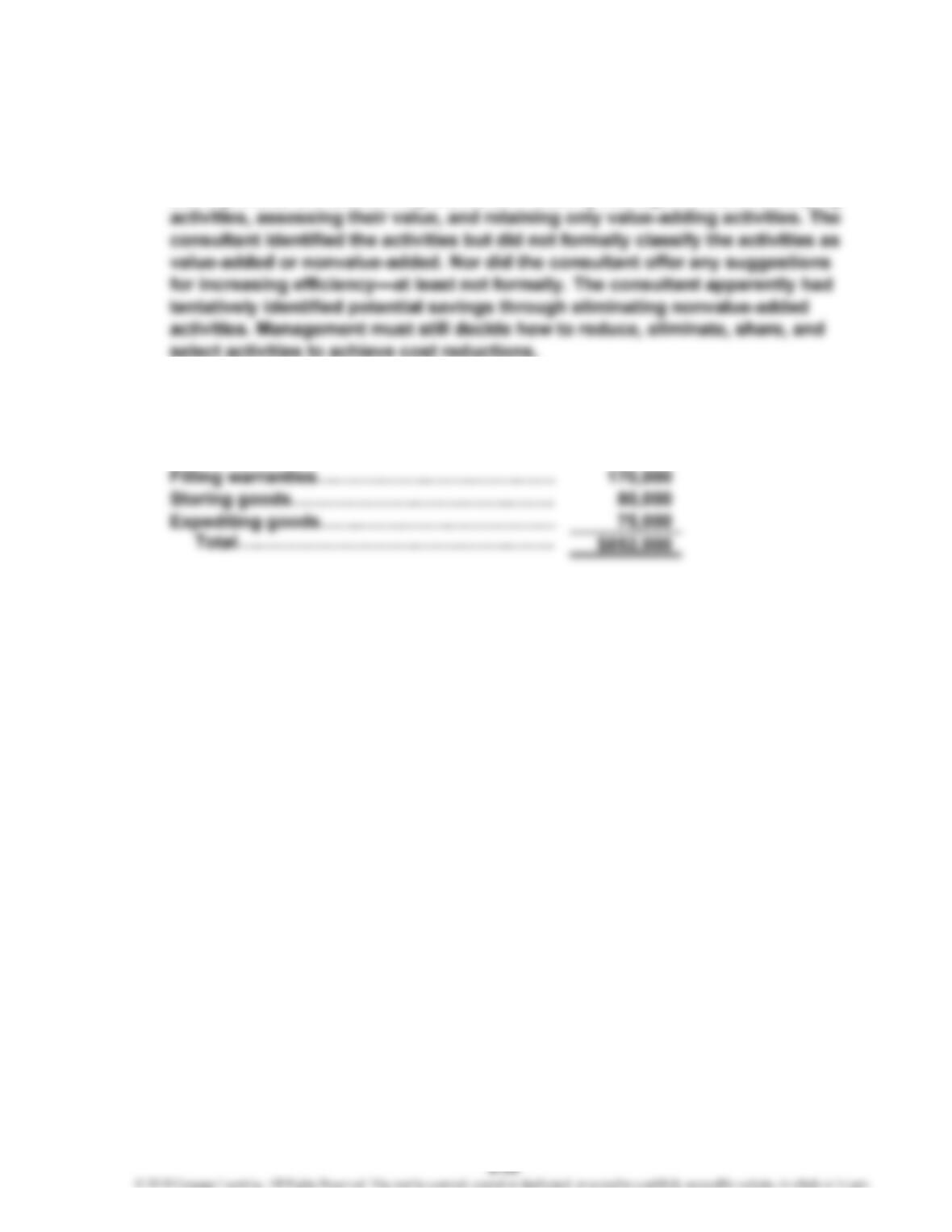
1. Activity-based management is a system-wide, integrated approach that focuses
management’s attention on activities. It involves two dimensions: a cost dimension
and a process dimension. Key elements in activity management are identifying
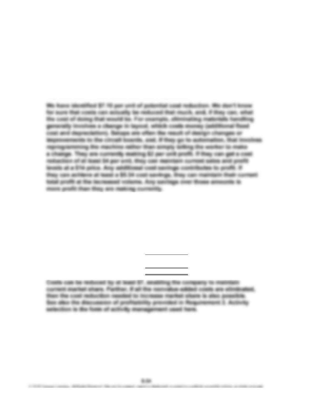
2. Setting up equipment……………………………
…
$125,000
Materials handling………………………………
…
180,000
Inspecting products……………………………… 122,000
Handling customer complaints………………… 100,000
…
…
CHAPTER 5 Activity-Based Costing and Management
P 5-60
(
Continued
)
Units produced and sold………………………………… 120,000 *
Potential unit cost reduction……………………………
…
$7.10 **
*$1,920,000/$16 (Total Cost/Unit Cost)
** $852,000/120,000 = $7.10
The consultant’s estimate of cost reduction was on target. Per-unit costs
can be reduced by at least $7, and further reductions may be possible if
improvements in value-added activities are possible.
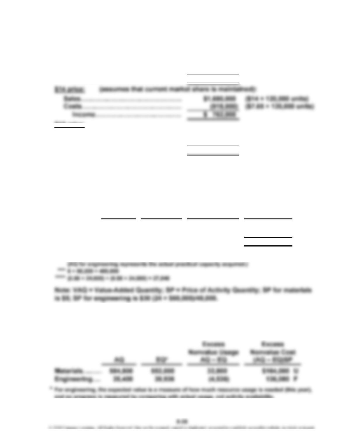
3. Unit cost to maintain sales = $14 – $4 = $10
Unit cost to expand sales = $12 – $4 = $8
Current cost = $16
Cost reduction to maintain = $16 – $10 = $6
Cost reduction to expand = $16 – $8 = $8
4. Total potential reduction:
$ 852,000 (from Requirement 2)
150,000 (by automating)
$1,002,000
÷ Units………………………………
…
120,000
Unit savings………………………… $ 8.35
CHAPTER 5 Activity-Based Costing and Management
P 5-60
(
Concluded
)
5. Current:
Sales………………………………………
…
$ 2,160,000 ($18 × 120,000 units)
Costs………………………………………
…
(1,920,000)
Income…………………………………
…
$ 240,000
$12 price:
Sales………………………………………
…
$ 2,160,000 ($12 × 180,000 units)
Costs………………………………………
…
(1,377,000) ($7.65 × 180,000 units)
Income…………………………………
…
$ 783,000
*
$16.00 – $8.35 = $7.65
The $12 price produces the greatest benefit.
P 5-61
1. Nonvalue-added usage and costs, 20X1:
Nonvalue Usage Nonvalue Cost
AQ*
V
AQ**
A
Q – VAQ (AQ – VAQ)SP
Materials……
…
600,000 480,000 120,000 $ 600,000
Engineering…
…
48,000 27,840 20,160 604,800
$1,204,800
*
1.25 × 6 × 80,000 = 600,000
**
(4 × 6,000) + (10 × 2,400) = 48,000
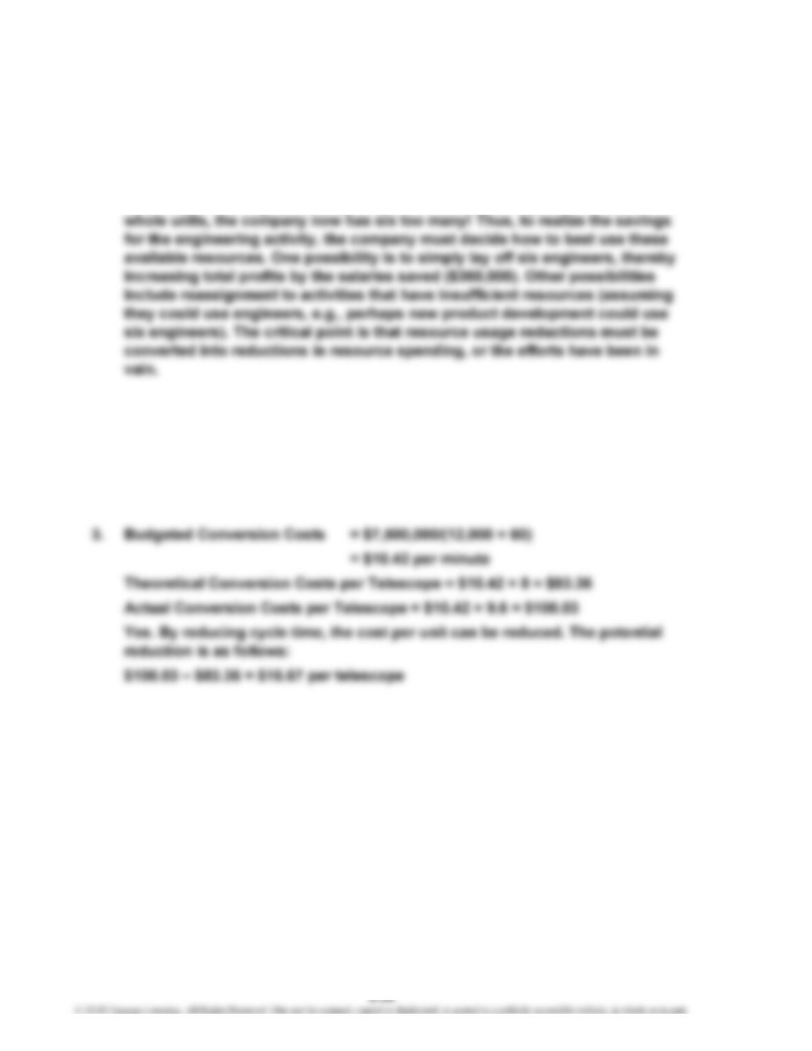
2. Expected values for the coming year (20X2):
Materials: EQ = 480,000 + 0.60(120,000) = 552,000 pounds
Engineering: EQ = 27,840 + 0.60(20,160) = 39,936 engineering hours
A
…
…
***
** ****
*
…
…
…
CHAPTER 5 Activity-Based Costing and Management
P 5-61 (Concluded)
The company failed to meet the materials standard but beat the engineering
standard. The engineering outcome is of particular interest. The actual usage
of the engineering resource is 35,400 hours, and activity availability is 48,000.
Thus, the company has created 12,600 hours of unused engineering capacity.
Each engineer brings a capacity of 2,000 hours. Since engineers come in
P 5-62
1. Theoretical Velocity = 90,000/12,000 hours = 7.5 telescopes per hour
Theoretical Cycle Time = 60/7.5 telescopes = 8 minutes per telescope
2. Actual Velocity = 75,000/12,000 hours = 6.25 telescopes per hour
Actual Cycle Time = 60/6.25 telescopes = 9.6 minutes
CHAPTER 5 Activity-Based Costing and Management
Case 5-63
1. Shipping and warehousing costs are currently assigned using tons of paper
produced, a unit-based measure. Many of these costs, however, are not driven b
y
2. The new method proposes assigning the costs of shipping and warehousing
separately for the low-volume products. To do so requires three cost assignments:
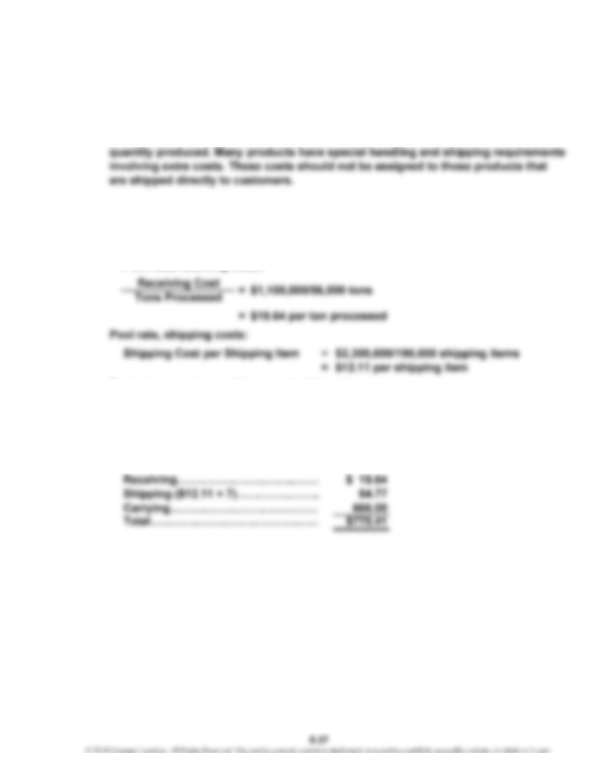
receiving, shipping, and carrying. The cost drivers for each cost are tons processed,
items shipped, and tons sold.
Pool rate, carrying cost (an opportunity cost):
Carrying Cost per Year (LLHC) = 25 × $1,665 × 0.16
= $6,660
Carrying Cost per Ton Sold = $6,660/10 = $666
Shipping and warehousing cost per ton sold:
CASES
CHAPTER 5 Activity-Based Costing and Management
Case 5-63 (Concluded)
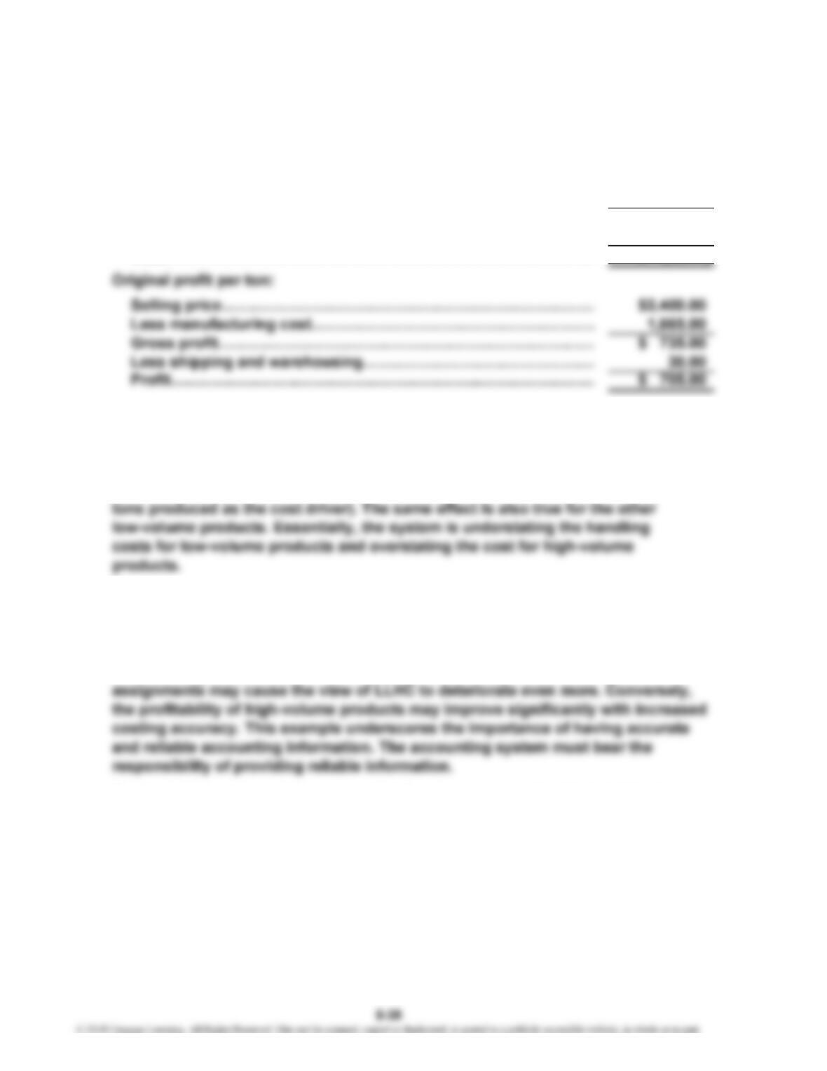
3. Profit analysis:
Revised profit per ton (LLHC):
Selling price………………………………………………………………
…
$2,400.00
Less manufacturing cost………………………………………………
…
1,665.00
Gross profit………………………………………………………………
…
$ 735.00
Less shipping and warehousing………………………………………
…
770.41
Loss………………………………………………………………………… $ (35.41)
The revised profit, reflecting a more accurate assignment of shipping and
warehousing costs, presents a much different picture of LLHC. The product is,
in reality, losing money for the company. Its earlier apparent profitability was
attributable to a subsidy being received from the high-volume products (by
spreading the special shipping and handling costs over all products, using
4. The decision to drop some high-volume products and emphasize low-volume
products could clearly be erroneous. As LLHC has demonstrated, its apparent
profitability is attributable to distorted cost assignments. A significant change in
the image of LLHC was achieved by simply improving the accuracy of shipping
and handling costs. Further improvements in accuracy in the overhead
5. Ryan’s strategy changed because his information concerning the individual
products changed. Apparently, the accounting system was undercosting the
low-volume products and overcosting the high-volume products. Once better
information was available, Ryan was able to respond better to competitive
conditions.
…
…
…
…
CHAPTER 5 Activity-Based Costing and Management
Case 5-64
1. Disagree. Chuck is expressing an uninformed opinion. He has not spent the
effort to find out exactly what activity-based management and costing are
2. and 3.
At first glance, it may seem strange to even ask if Chuck’s behavior is unethical.
After all, what is unethical about expressing an opinion, albeit uninformed? While
offering uninformed opinions or recommendations may be of little consequence
in many settings, a serious issue arises when a person’s expertise is relied upon
by others to make decisions or take actions that could be wrong or harmful to
themselves or their organizations. This very well may be the case for Chuck’s
setting, and his behavior may be labeled professionally unethical.