43
DISCRETE
PROBABILITY
DISTRIBUTIONS
4.1 xPr X x
0 .72
4.3
Var(X) E(X
2
)
P
2
4.4 xF
x
0 0
4.7 We have
10 0 10 1 10 2
110 10 9
21 45CC C
u
u ,, ,
44 CHAPTER 4/DISCRETE PROBABILITY DISTRIBUTIONS
4.9 We wish to compute
4.14 Let X1 the number of inner-city newborns with HIV-positive test results. We have that
4.15
Pr X
1
t5
1Pr X
1
d4
. We use the pbinom command in R to compute
1Pr X
1
d4
. We have
4.16 Since n t500 100, and p ..008 01, we can use the Poisson approximation
Y1
to the binomial
CHAPTER 4/DISCRETE PROBABILITY DISTRIBUTIONS 45
4.17 Let X2 = number of mixed urban/suburban hospital infants that are positive for the HIV virus. We have
that
4.18
Pr X
2
t5
1Pr X
2
d4
. We use the pbinom command in R to compute
1Pr X
1
d4
as follows:
4.19 We use a Poisson approximation with
P
np 500 11
5006
§
©
¨
·
¹
¸ 1.1
. Therefore,
4.20 Let X3 = number of mixed suburban/rural hospital infants that test positive for HIV virus. We have that
4.21
Pr X
3
t5
1Pr X
3
d4
. We use the pbinom command in R to compute
1Pr X
3
d4
as follows:
46 CHAPTER 4/DISCRETE PROBABILITY DISTRIBUTIONS
4.23 The distribution of the number of gonorrhea cases that occurred over a 3-month period is approximated
4.24 We have that Pr(k episodes of otitis media over time t) is given by
4.26 From Problem 4.24, Pr(1 sibling has 3+ episodes of otitis in 2 years) = .62. Thus, if the number of
CHAPTER 4/DISCRETE PROBABILITY DISTRIBUTIONS 47
4.30 The probability that a hypertensive is being treated appropriately and is complying with the treatment is
Pr(hypertensive is told he or she has high blood pressure)
4.31 Pr(hypertensive knows he or she has high blood pressure) 1
2. We want
4.32 If the rates are each decreased to 40%, then .. .6 216 216%
3
of hypertensives will be appropriately
treated as opposed to .. .5 125 12 5%
3
. Thus, if the current annual mortality rate for untreated
4.33 We have
48 CHAPTER 4/DISCRETE PROBABILITY DISTRIBUTIONS
4.34 Pr(3 or more )1Pr (2 or less +)
4.35 We know that X can only take on the values 0, 1, or 2.
Pr Pr 2 Pr
0
negatives negative at time 0
Thus, the probability of distribution X is
XPr(X)
CHAPTER 4/DISCRETE PROBABILITY DISTRIBUTIONS 49
4.37 Variance of
22
XEX
P
4.38 The probability that an infant will be disease-free at the end of 6 months
1875
4.39 There are 2300 infants who have not had otitis media by the end of the 3rd month of life of which
4.40 Let
X
the number of siblings who develop otitis media in the first 6 months of life. X is binomially
4.43 We refer to Table 1 under n 18 , p .1 . We have
4.44 Pr(rat will die in an 8-hour period)
Pr
(rat will die in the first 4 hours)
Pr
Pr
50 CHAPTER 4/DISCRETE PROBABILITY DISTRIBUTIONS
4.48 If
X
number of cases of Down’s syndrome, then X follows a Poisson distribution with
P
19 . To
P
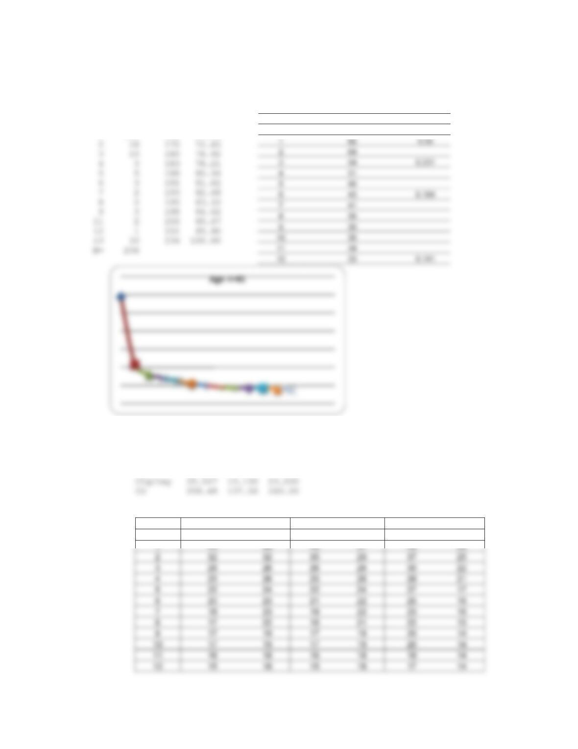
4.55 First, we create a table showing the values of the variable “Day_abs”.
TallyforDiscreteVariables:Day_abs
Day_abs Count
0 13
1 15
CHAPTER 4/DISCRETE PROBABILITY DISTRIBUTIONS 51
From our table, we can see that the estimated probability of remaining abstinent for 1, 3, 6 and 12 months,
respectively, is 0.35, 0.231, 0.184, and 0.141.
Month
OVERALL LIFE TABLE
Resumed Count CumCnt CumPct
0 13 13 5.56
1 139 152 64.96
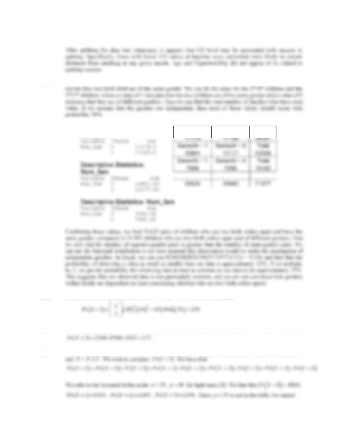
4.52 For each of the variables mentioned, we will consider two groups. For Age, Number of Cigarettes, and
CO level, we consider those with values above and below the median.
Variable Mean StDev Median
Age 42.248 12.313 41.000
SUBGROUP LIFE TABLES
Month Age <=41 Age > 41 Cig <= 23 Cig > 23 CO <= 260 CO > 260
0 118 116 121 113 116 111
Month # Remaining Abstinent Proportion
0 234
52 CHAPTER 4/DISCRETE PROBABILITY DISTRIBUTIONS
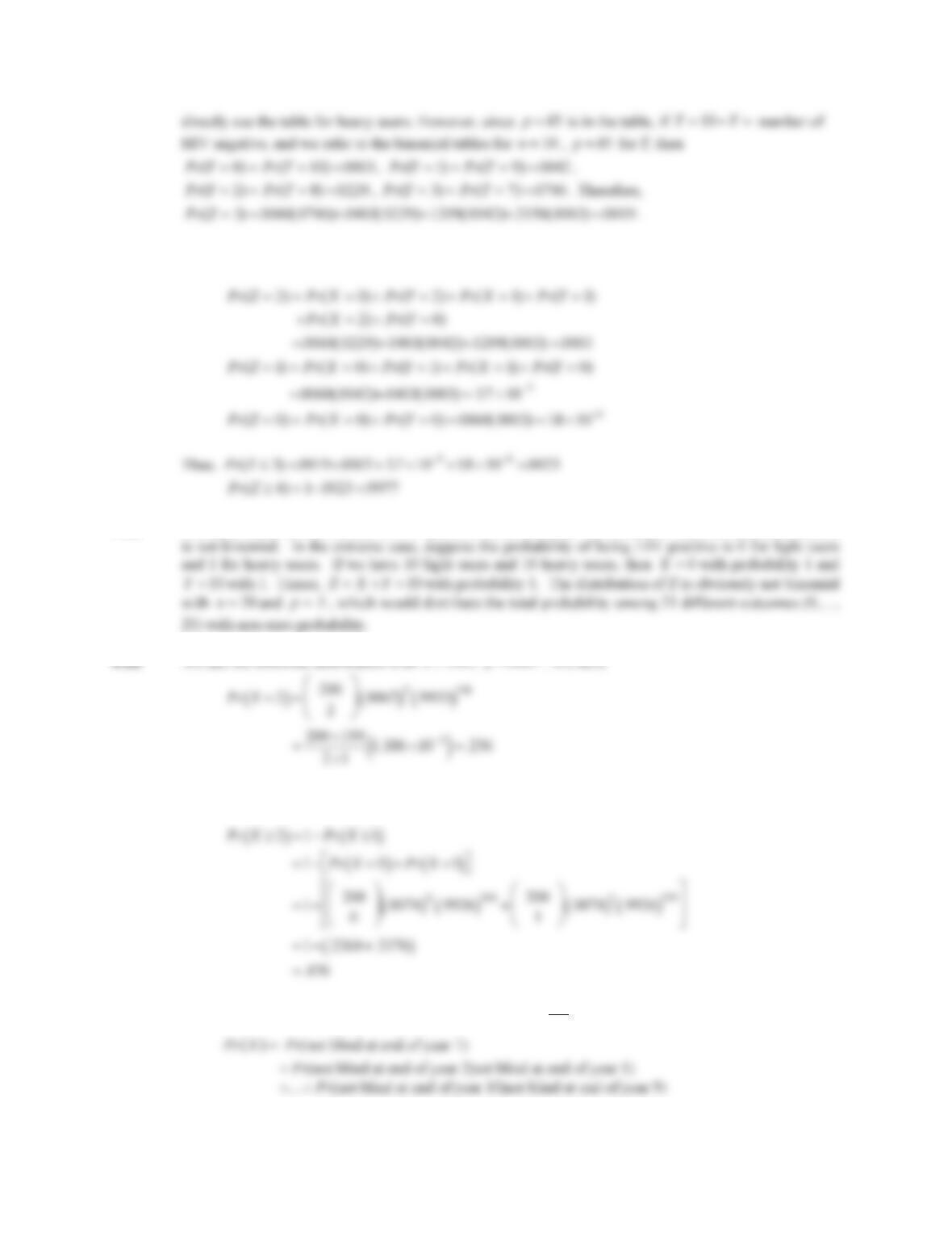
4.53 One option is to create an indicator variable ‘13Same’ to indicate, within each family type, whether or
Descriptive Statistics:
Num_fam
4.54 We use the binomial distribution with n 5, p .40 . We wish to compute
4.55 We wish to compute Pr X t
3. We refer to the binomial table (Table 1) under n 5, p .40 , and find
4.56 Let
X
number of light users who are HIV positive, Y number of heavy users who are HIV positive,
X
Same13 = 1 Same13 = 0 Total
CHAPTER 4/DISCRETE PROBABILITY DISTRIBUTIONS 53
4.57 We wish to compute Pr PrZZt
d
41 3. We have Pr Z
3 0019. from Problem 4.56.
4.58 The distribution of the number of HIV positive is not binomial. A mixture of two binomial distributions
4.60 We use the binomial distribution with n 200 , p .0074 . We wish to compute
4.61 Let
X
event that a 30-year-old male IDDM patient will not become blind over 10 years.