54 CHAPTER 4/DISCRETE PROBABILITY DISTRIBUTIONS
4.62 Suppose a person is followed for n years. Using a similar argument as given in the answer to Problem
4.76,
4.64 Let
X
number of cardiac deaths on the day of the earthquake. If the cardiac death rate in the previous
week continued to hold on the day of the earthquake, then X would follow a Poisson distribution with
mean
P
15 6.. Thus,
4.65 To judge whether 51 cardiac deaths is an unusual occurrence we wish to compute
CHAPTER 4/DISCRETE PROBABILITY DISTRIBUTIONS 55
4.66 We wish to find the number of deaths k such that
4.67 We wish to find the smallest value k such that
4.68 We wish to find the smallest value k such that
4.69 We wish to find
Pr
X
4 where X is a mixture of 2 Poisson distributions with parameters 2.0 on 345
normal pollution days and 4.0 on 20 high pollution days. Therefore
4.70 Let X = number of emergency room admissions on a given day. We wish to find the smallest k such that
56 CHAPTER 4/DISCRETE PROBABILITY DISTRIBUTIONS
k
Pr 2Xk
P
d
Pr 4Xk
P
d
Pr Xkd
4 0.947 0.629 0.930
4.71 We calculate the probability of not having an abortion over the 30 year period. This is given by
4.73 We assume that the observed number of abortions is Poisson distributed with parameter
P
54 233,. We
wish to compute Pr X d
16 539 54 233,,
P
. Unfortunately, the value of
P
is too large to be handled by
4.74-4.79
To begin, we use R to create variables that tell us whether each twin pair has a positive or negative score
for each measure of bone density:
CHAPTER 4/DISCRETE PROBABILITY DISTRIBUTIONS 57
4.74-4.75
> boneden_sorted_ls<-boneden[order(-abs(boneden$pyr2-boneden$pyr1)), ]
> boneden_sorted_ls$top20<-c(rep(1, 20), rep(0, 21))
> addmargins(table(boneden_sorted_ls$lsDif, boneden_sorted_ls$top20))
0 1 Sum
-1 11 17 28
4.76-4.77
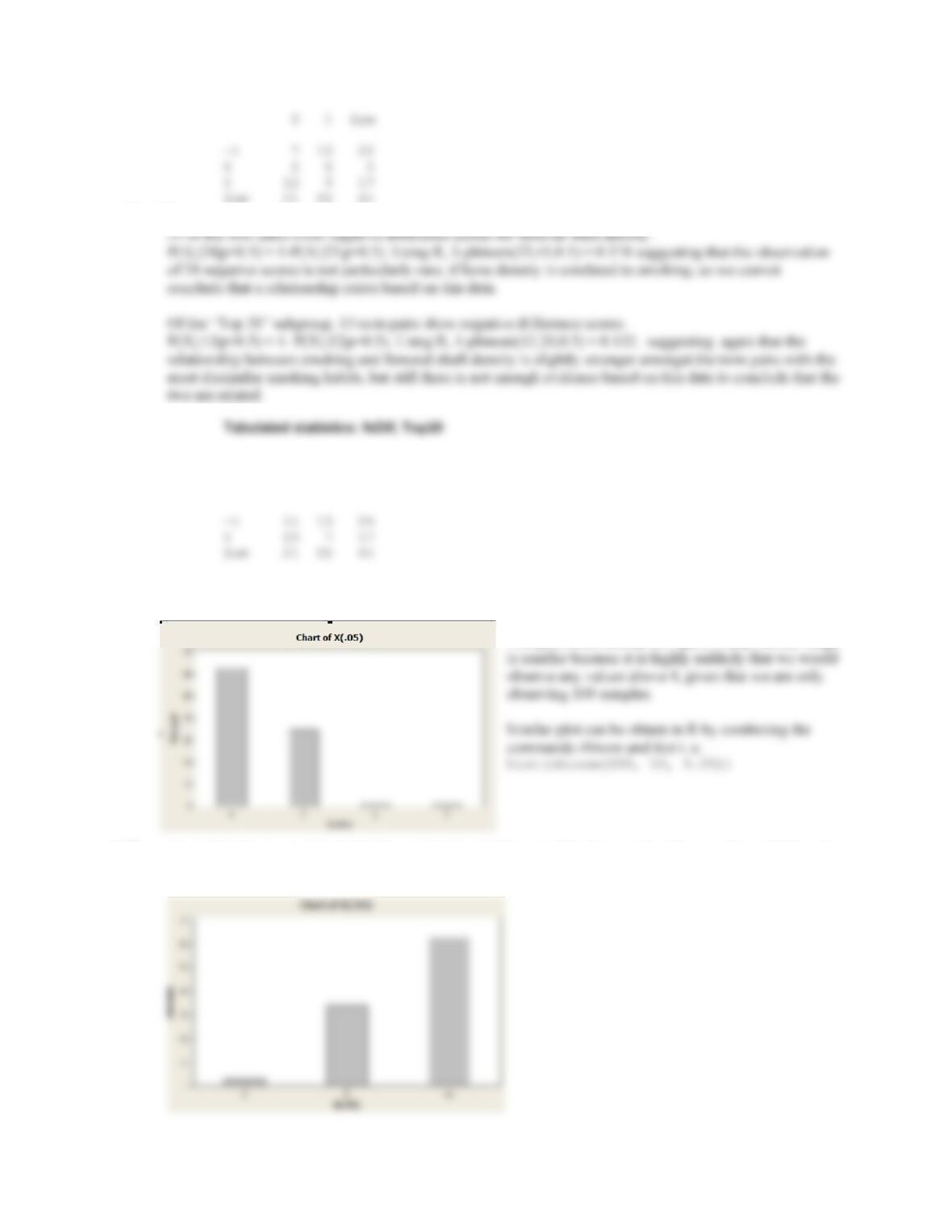
22 of the twin pairs show negative difference scores for femoral neck density, though only 39 had either a
positive or negative score. We will ignore those who had a difference score of 0. In this case, we would
58 CHAPTER 4/DISCRETE PROBABILITY DISTRIBUTIONS
Sum 21 20 41
4.78-4.79
Rows: fsDif Columns: Top20
0 1 Sum
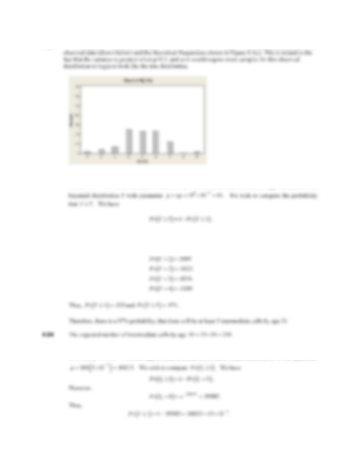
4.80 Using the command “Calc – Random Data – Binomial” in MINITAB, it is easy to draw random samples.
Here is a sample frequency distribution from 100 random draws with p=0.05.
This plot looks similar to Figure 4.4(a), but our range
4.81 Again, this histogram has similar shape to the one in Figure 4.4(b), but we only observe values of 8,9, and
10 in our random sample.
CHAPTER 4/DISCRETE PROBABILITY DISTRIBUTIONS 59
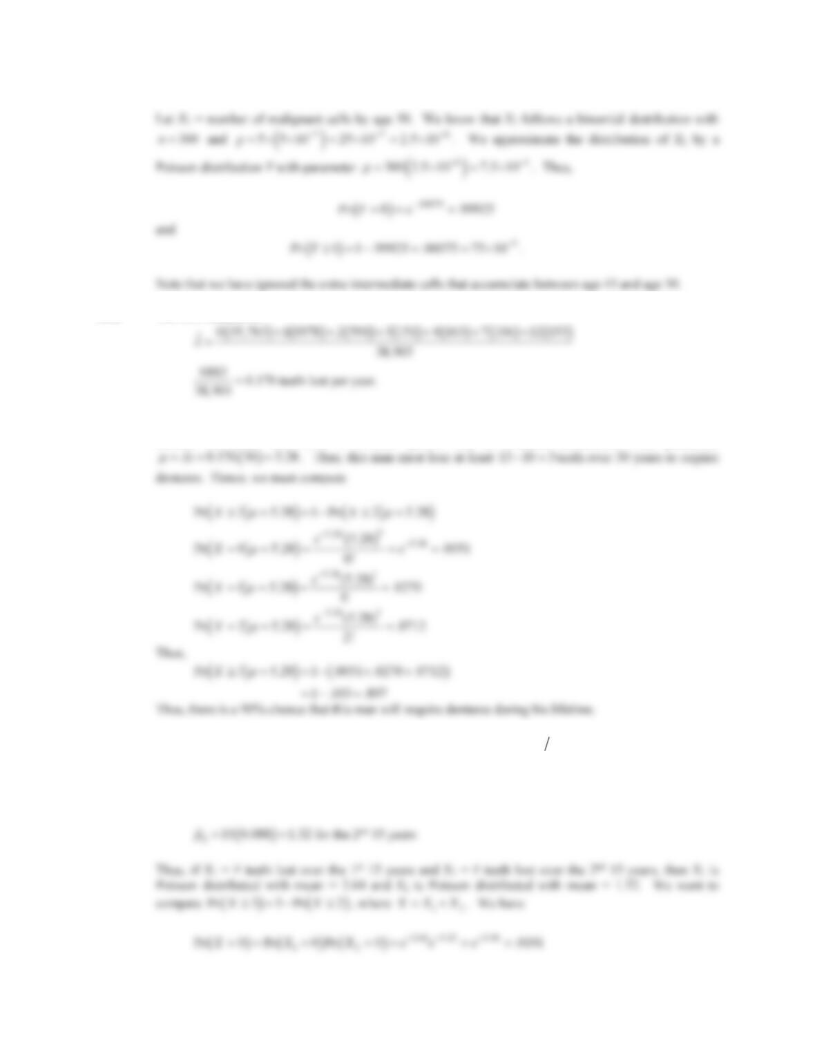
4.82 For the frequency distribution associated with n=10 and p=0.50, we find the most discrepancy between our
4.83 The number of intermediate cells by age 21 (X) follows a binomial distribution with parameters 8
10n
and 7
10p
. However, because 100ntand 0.01pd, we can use the Poisson approximation to the
Referring to Table 2 (Appendix, text), we have that
0 .0000
Pr Y
4.85 Let X1 = number of malignant cells by age 46. We know that X1 follows a binomial distribution with
300n , 7
510p
u . We will approximate this distribution by a Poisson distribution Y1 with parameter
60 CHAPTER 4/DISCRETE PROBABILITY DISTRIBUTIONS
4.86 The best estimate is
4.87 We calculate the proportion of men with 10 or fewer teeth remaining in 2016. For this purpose, the
number of teeth lost over a 30-year period (X) is Poisson distributed with parameter
4.88 We have
ˆ0.176
O
teeth lost per year for the 1st 15 years and ˆ0.176 2 0.088
O
teeth lost per year for
the 2nd 15 years. Thus,
1
ˆ15 0.176 2.64
P
for the 1st 15 years
CHAPTER 4/DISCRETE PROBABILITY DISTRIBUTIONS 61
4.91 Let us create new variables W and Z, representing the number of weekday and weekend admissions in a
given week, respectively. W is a Poisson random variable with μ= 10 = (5 days x 2 per day) , and Z is a
4.94 Note that the high SES regions (Tracts A and G) produce 10,000 births per year, with an expected number
of birth defects of 10,000 x 50/100,000 = 5.
62 CHAPTER 4/DISCRETE PROBABILITY DISTRIBUTIONS
4.95 As in 4.102, the high SES regions (Tracts A and G) produce 10,000 births per year, with an expected
number of birth defects of 10,000 x 50/100,000 = 5.
4.96 The probability of an in-flight medical emergency (IFM) on one flight is given by:
4.97 Let Y = number of IFM’s over 20 years. We could use the Poisson approximation to the binomial
4.99 The probability that a subject is eligible and willing to participate is p = 0.031(0.52) = 0.01612.
Let X = number of subjects eligible and willing to participate. X is binomially distributed with n = 100 and
p = 0.01612. Also,
CHAPTER 4/DISCRETE PROBABILITY DISTRIBUTIONS 63
4.100 Let Y = number of people out of 1000 who are eligible and willing to participate. We wish to compute:
4.101 We will use a binomial distribution with n=20 and p=0.16. We will compute
4.102 We wish to compute Pr(X3)= 1 – Pr(X2)
4.103 Let Y = number of patients who do not develop arrhythmia and have a complete response.
Z = number of patients who develop arrhythmia and have a complete response.
Thus, Y+Z=3
64 CHAPTER 4/DISCRETE PROBABILITY DISTRIBUTIONS
4.104 From Table 2, we find that if X is Poisson distributed with parameter μ=12, then
4.105 Let X be the number of patients who survive for >= 18 months. Based on the result in 4.104, X will
be binomially distributed with parameters n = 5 and p = .063. We wish to compute P(X 3).