CHAPTER 3 Cost Behavior
E 3-39
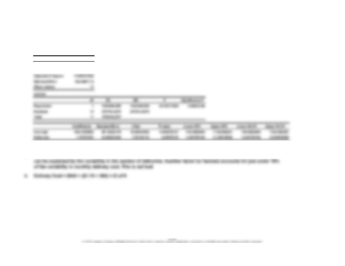
1. SUMMARY OUTPUT
Multiple R 0.917226463
R Square 0.841304384
2. Delivery Cost = $942 + ($1.79 × Number of Deliveries)
3. The R² is 0.841, or 84.1%. In other words, 84.1% of the variation in the monthly cost of delivery from month to month
Regression Statistics
CHAPTER 3 Cost Behavior
P 3-40
1. a. Mixed cost
b. Variable cost
c. Variable cost
2. a. While the contract stays the same ($150 per month plus $15 per hour of technical
time), the company’s need for computer technical help is so stable that the same
number of hours are required each month. Now, the cost is essentially fixed.
b. The company drives the vehicles on identical trips each month. Thus, the mileage
and type of trip (highway versus in town) never vary. Now, the cost is essentially
g. If the individuals working behind the counter are assured that their complete shift
would be worked once they arrive, the cost would be a step cost (assumes more
counter help could be called in if demand rose).
PROBLEMS
CHAPTER 3 Cost Behavior
P 3-41
a. This must be the high-low method because she has only two data points (one for
each year).
P 3-42
a. Variable cost
b. Committed fixed cost
CHAPTER 3 Cost Behavior
P 3-43
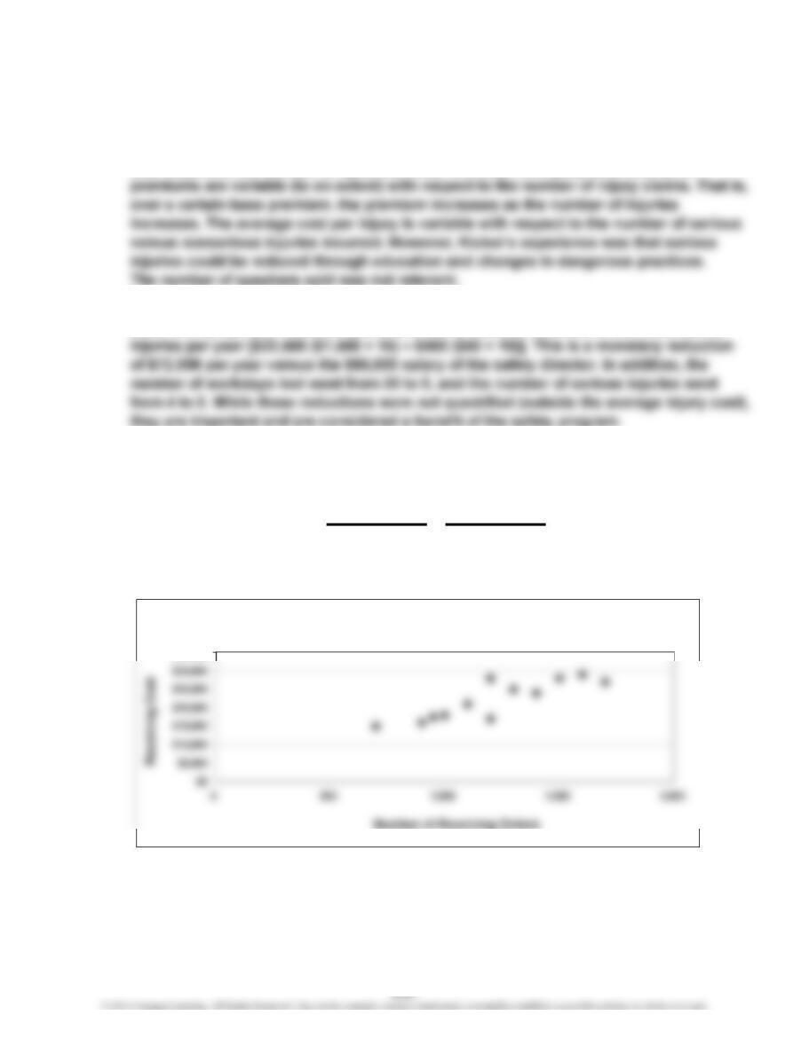
1.
2. Using the high-low method:
Variable Receiving Cost = ($27,000 – $15,000)/(1,700 – 700) = $12
Fixed Receiving Cost = $15,000 – ($12 × 700) = $6,600
Scattergraph of Receiving Activity
$30,000
$35,000
CHAPTER 3 Cost Behavior
P 3-44
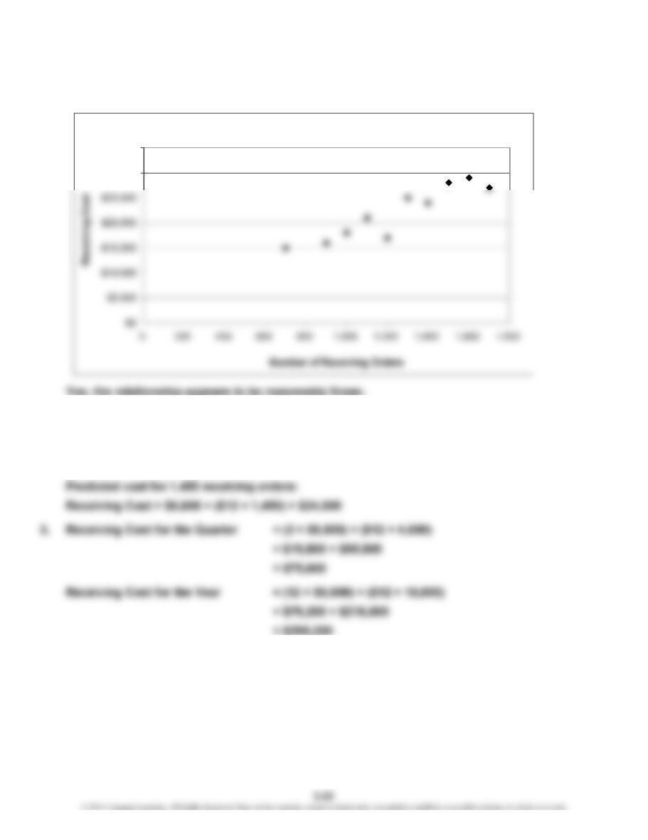
1. Receiving Cost = $3,212 + ($15.15 × Number of Receiving Orders)
2. Receiving Cost = $3,212 + ($15.15 × 1,450) = $25,180
P 3-45
1. Salaries:
Senior accountant—fixed
Office assistant—fixed
P 3-45 (Continued)
2. Internet and software subscriptions:
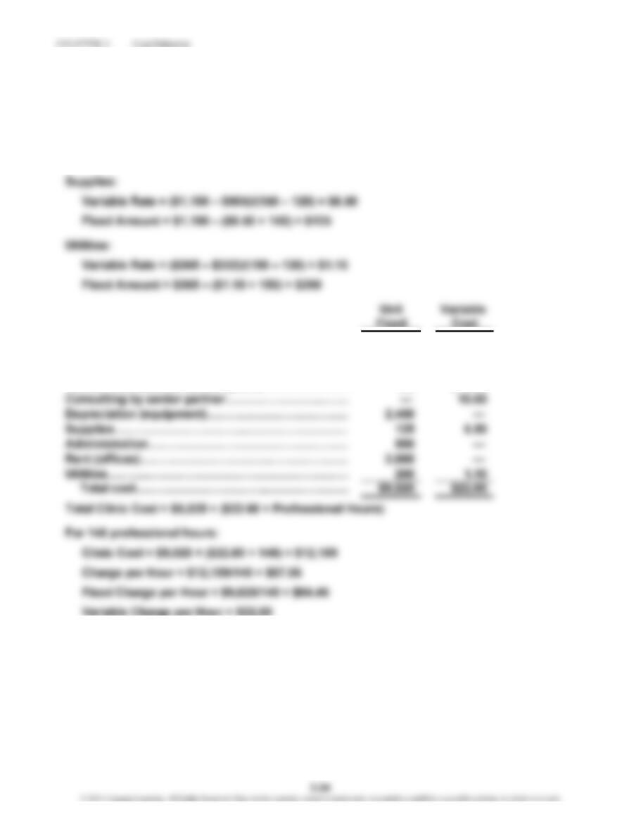
Variable Rate = ($850 – $700)/(150 – 120) = $5
Fixed Amount = $850 – ($5 × 150) = $100
3. Salaries:
Senior accountant……………………………………
…
$2,500 —
Office assistant………………………………………… 1,200 —
Internet and software subscriptions…………………
…
100 $ 5.00
…
4. For 170 professional hours:
Charge per Hour = ($9,025/170) + $22.60 = $75.69
The charge drops because the fixed costs are spread over more professional
hours.
P 3-46
1. Committed resource charges: monthly fee, activation fee, cancellation fee
(if triggered by contract cancellation prior to 1 year)
Flexible resource charges: all additional charges for airtime, long distance,
and roaming.
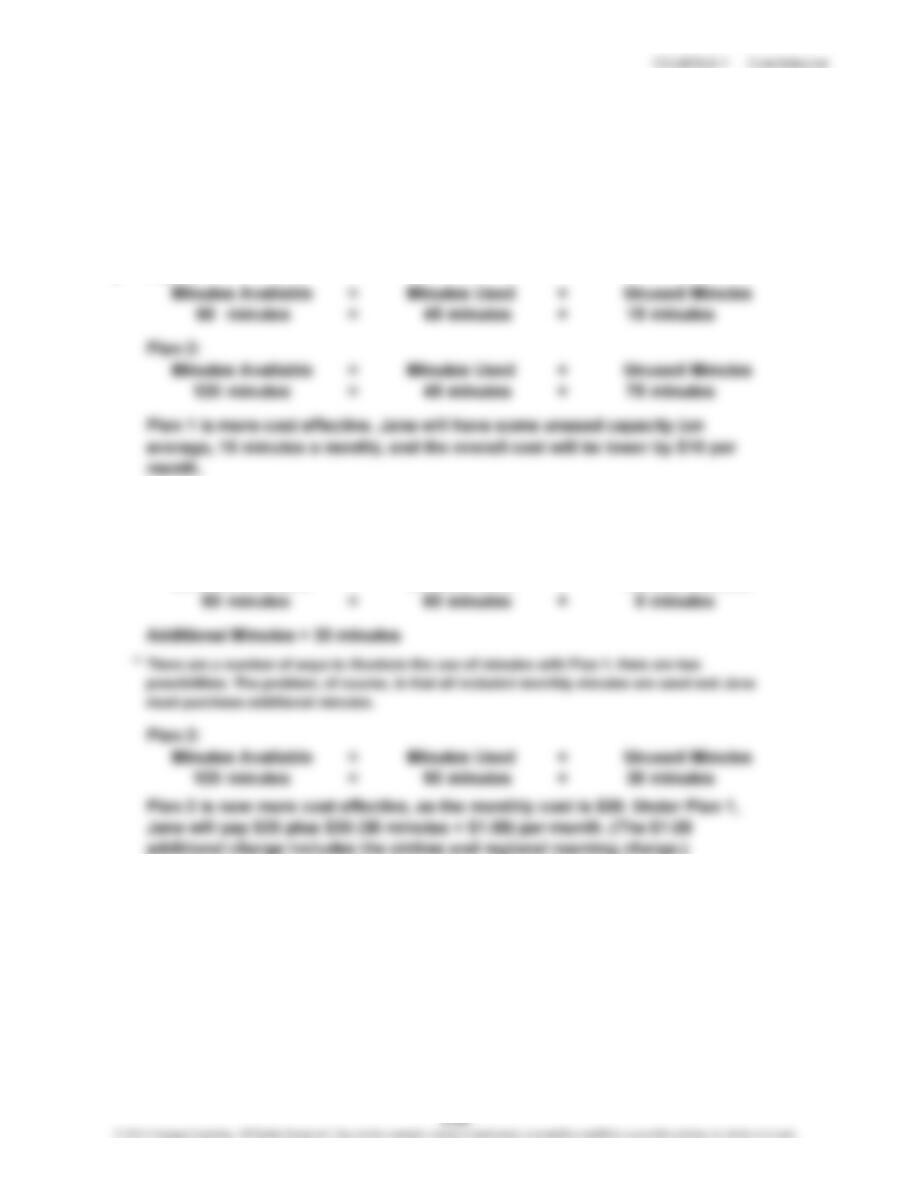
2. Plan 1:
3. Plan 1:*
=+
60 minutes = 90 minutes + (30) minutes
=+
4. Results of students’ analyses will vary.
Minutes Available Minutes Used Unused Minutes
Minutes Available Minutes Used Unused Minutes
CHAPTER 3 Cost Behavior
P 3-47
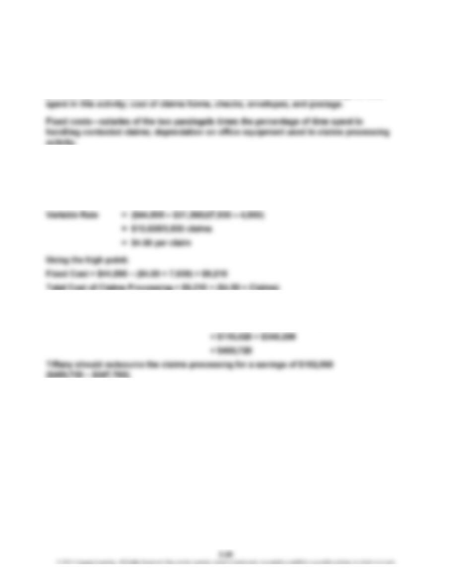
1. Variable costs—salary of the two paralegals times the percentage of time spent in
processing uncontested claims; salary of the accountant times the percentage of time
2. The independent variable is number of claims; the dependent variable is cost of claims
processing.
3. The low point is March with $31,260 cost and 4,900 claims; the high point is June with
$44,895 cost and 7,930 claims.
4. Cost of Outsourcing = $4.60 × 75,600 = $347,760
Cost of Processing In-House = (12 × $9,210) + ($4.50 × 75,600)
CHAPTER 3 Cost Behavior
P 3-48
1. The state unemployment insurance premiums and the average cost per injury are fixed
with respect to the number of speakers sold. The state unemployment insurance
2. Yes, the safety program paid for itself. There was a $50,000 reduction in annual cost of
state unemployment insurance premiums and a $22,000 reduction in the total cost of
P 3-49
1. Results of regressions:
10 Months’ 12 Months’
Data Data
Intercept…………………
…
3,212 3,820
Slope………………………
…
15.15 15.10
R²…………………………
…
0.85 0.75
2.
Scattergraph of Receiving Activity—12 Month’s Data
$35,000

CHAPTER 3 Cost Behavior
P 3-49 (Continued)
The point for the 11th month (1,200 receiving orders and $28,000 total receiving cost) appears to be an outlier. Since the
3. Results for the method of least squares after dropping Month 11.
SUMMARY OUTPUT
Regression Statistics
Multiple R 0.926737002
R Square 0.85884147
Adjusted R Square 0.843157189
P 3-49 (Continued)
The regression run on the 11 months of data from “typical” months appears to be better
than the one for all 12 months. R² is higher for the regression without the outlier
P 3-50
1.
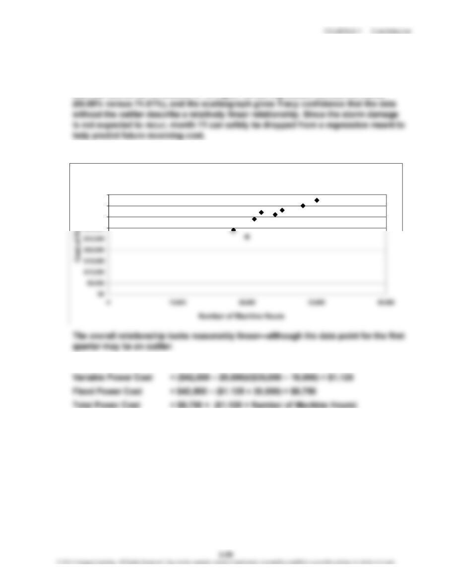
2. Using the high-low method:
Scattergraph of Power Cost
$30,000
$35,000
$40,000
$45,000
P 3-50 (Continued)
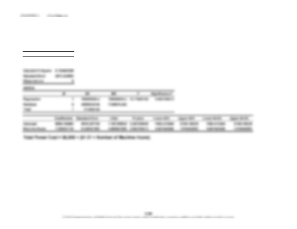
3. Output of regression program:
SUMMARY OUTPUT
Regression Statistics
Multiple R 0.893359672
R Square 0.798091504
R² is 0.798, or 79.8% This is not bad; however, a little more than 20% of the variance in the dependent variable
(power cost) is not explained by the independent variable (machine hours).
CHAPTER 3 Cost Behavior
P 3-50 (Continued)
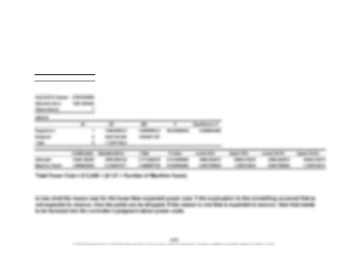
4. The output of a regression program after quarter 1 (20,000, $26,000) has been dropped.
SUMMARY OUTPUT
Regression Statistics
Multiple R 0.957883502
R Square 0.917540803
This regression looks better in terms of R². The R² for this regression is 0.92, or 92%. By dropping the outlier, the
explanatory power of machine hours is much improved. However, the controller should first carefully examine Quarter 1
CHAPTER 3 Cost Behavior
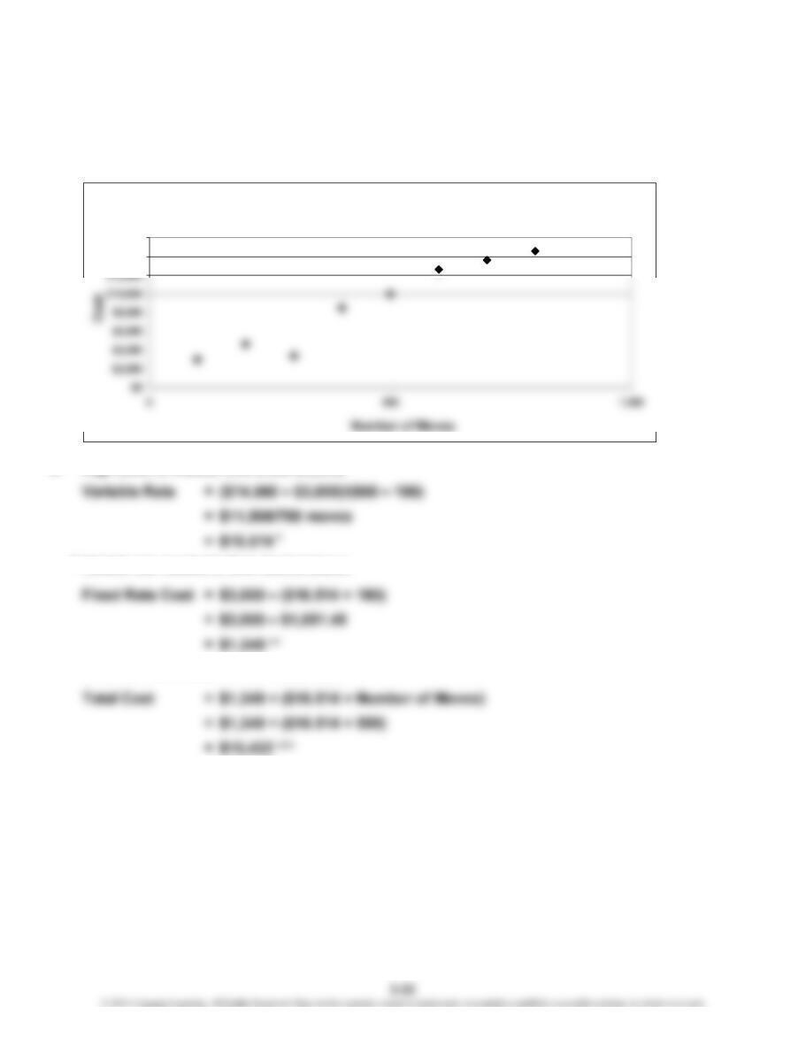
P 3-51
1. The scattergraph provides evidence for a linear relationship, but the observation for
300 moves may be an outlier.
2. High (800, $14,560); Low (100, $3,000)
*Variable rate rounded to three decimal places.
** Total fixed cost rounded to the nearest dollar.
*** Total cost rounded to the nearest dollar.
Cost of Moving Materials
$14,000
$16,000
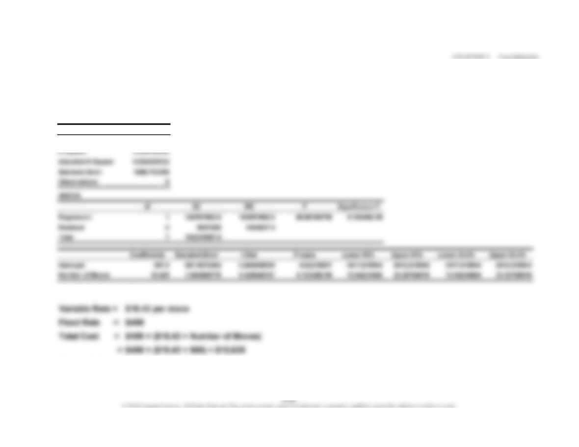
P 3-51 (Continued)
3. Output of the regression routine calculated by a spreadsheet:
SUMMARY OUTPUT
Regression Statistics
Multiple R 0.96785846
Rounding the coefficients:
R² = 0.94 (rounded)
This says that 94% of the variability in the cost of moving materials is explained by the number of moves.
CHAPTER 3 Cost Behavior
P 3-51 (Continued)
4. Normally, we would prefer the least squares method since the data appear to be linear.
However, the third observation may be an outlier. If the third observation (300 moves
CHAPTER 3 Cost Behavior
Case 3-52
1. The order should cover the variable costs described in the cost formulas.
These variable costs represent flexible resources.
Materials ($94 × 20,000)……………………………………………………
…
$1,880,000
2. The coefficients of determination indicate the reliability of the cost formulas.
Of the four formulas, overhead activity may be a problem. A coefficient of
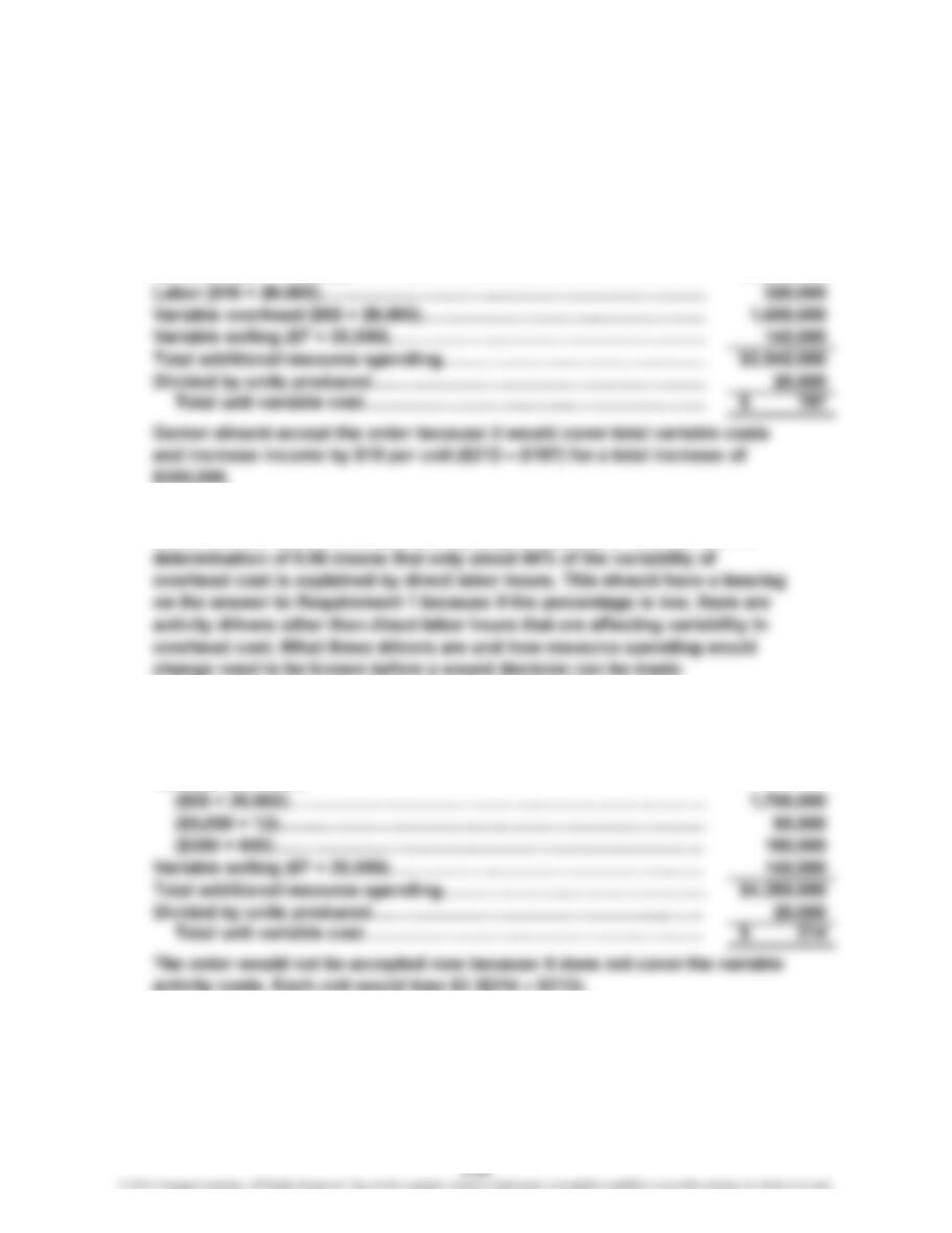
3. Resource spending attributable to order:
Materials ($94 × 20,000)…………………………………………….………
…
$1,880,000
Labor ($16 × 20,000)…….…………………………………….…..…………
…
320,000
Variable overhead:
…
…
CASES
…
…
…
CHAPTER 3 Cost Behavior
Case 3-52 (Continued)
It would also be useful to know the step-cost functions for any activities that have
Case 3-53
1. Carl’s behavior is definitely unethical. He is stealing confidential information from
Kilborn and using it for unethical advantages. Kilborn would not approve of Carl’s
actions and would have a potential lawsuit against him for theft of information.
2. Assuming that the data were acquired illicitly, Bill’s instincts were on target. To hire
Carl in implicit exchange for the confidential information would be a violation of
integrity. As soon as Carl joined Brindon’s staff, Kilborn could have legal standing