1. Knowledge of cost behavior allows a manager to assess changes in costs that result from
changes in activity. This allows a manager to examine the effects of choices that change activity.
For example, if excess capacity exists, bids that at least cover variable costs may be totally
appropriate. Knowing what costs are variable and what costs are fixed can help a manager make
better bids and, ultimately, better business decisions.
4. Some account categories are primarily fixed or variable. Even if the cost is mixed, either the fixed
component or the variable component is relatively small. As a result, assigning all of the cost to
either a fixed or variable category is unlikely to result in large errors. For example, depreciation on
property, plant, and equipment is largely fixed. The cost of telephone expense for the sales office,
if it consisted primarily of long-distance calls, could be seen as largely variable (variable with
respect to the number of customers).
5. Committed fixed costs are those incurred for the acquisition of long-term activity capacity and are
7. Mixed costs are usually reported in total in the accounting records. How much of the cost is fixed
and how much is variable is unknown and must be estimated.
8. The cost formula for a strictly fixed cost has only a fixed cost amount. There is no variable rate
and no independent variable. For the depreciation example, the cost formula looks like this:
Depreciation per Year = $15,000
3COST BEHAVIOR
DISCUSSION QUESTIONS
A
selection of the two points is not left to judgment.
12. Because the scattergraph method is not restricted to the high and low points, it is
possible to select two points that better represent the relationship between activity and
costs, producing a better estimate of fixed and variable costs. The main advantage of the
high-low method is that it removes subjectivity from the choice process. The same line
will be produced by two different people.
13.
A
ssuming that the scattergraph reveals that a linear cost function is suitable, then the
method of least squares selects a line that best fits the data points. The method also
provides a measure of goodness of fit so that the strength of the relationship between
cost and activity can be assessed.
CHAPTER 3 Cost Behavior
3-1. c
3-2. e
3-3. b
MULTIPLE-CHOICE QUESTIONS
CHAPTER 3 Cost Behavior
CE 3-15
1. The cost formula takes the following form:
Total Cost = Fixed Cost + (Variable Rate × Number of Flash Drives)
The monthly fixed cost is the $15,000 cost of equipment depreciation, as it does not
vary according to the number of flash drives manufactured. The variable costs are
2. Expected fixed cost for next month is $15,000.
Expected variable cost for next month is:
CORNERSTONE EXERCISES
CHAPTER 3 Cost Behavior
CE 3-16
Step 1: Find the high and low points: The high number of employee hours is in March,
and the low number of employee hours is in August.
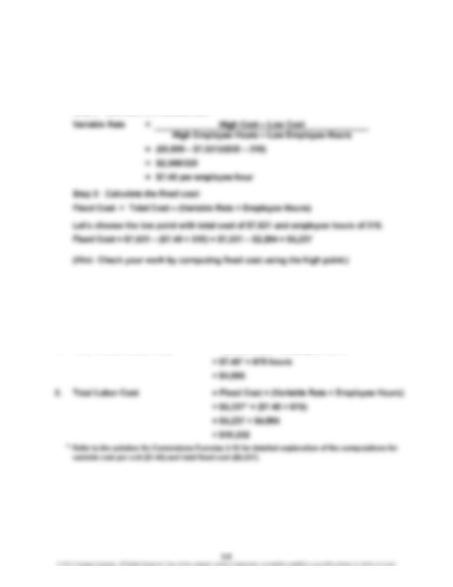
Step 2: Calculate the variable rate:
Step 4: Construct a cost formula:
If the variable rate is $7.40 per employee hour and fixed cost is $5,237 per month, then
the formula for total monthly labor cost is:
Total Labor Cost = $5,237 + ($7.40 × Employee Hours)
CE 3-17
1. Total Variable Labor Cost = Variable Rate × Employee Hours
CHAPTER 3 Cost Behavior
CE 3-18
1. Total Variable Labor Cost = Variable Rate × Employee Hours
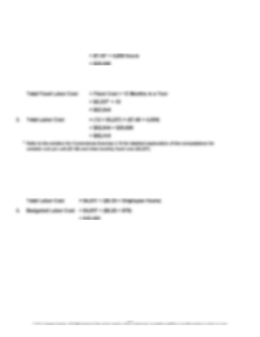
2. There’s a trick here; the cost formula is for the month, but we are being asked to budget
labor cost for the year. So, we will need to multiply the fixed cost for the month by 12
(the number of months in a year).
CE 3-19
1. The fixed cost and the variable rate are given directly by regression.
Fixed Cost = $4,517
Variable Rate = $8.20
2. The cost formula is:
CHAPTER 3 Cost Behavior
E 3-20
a. Power to operate a drill (to drill holes in the wooden frames of the futons)—
Variable cost
b. Cloth to cover the futon mattress—Variable cost
E 3-21
1.
EXERCISES
Truck Depreciation
200,000
250,000
CHAPTER 3 Cost Behavior
E 3-21 (Continued)
2.
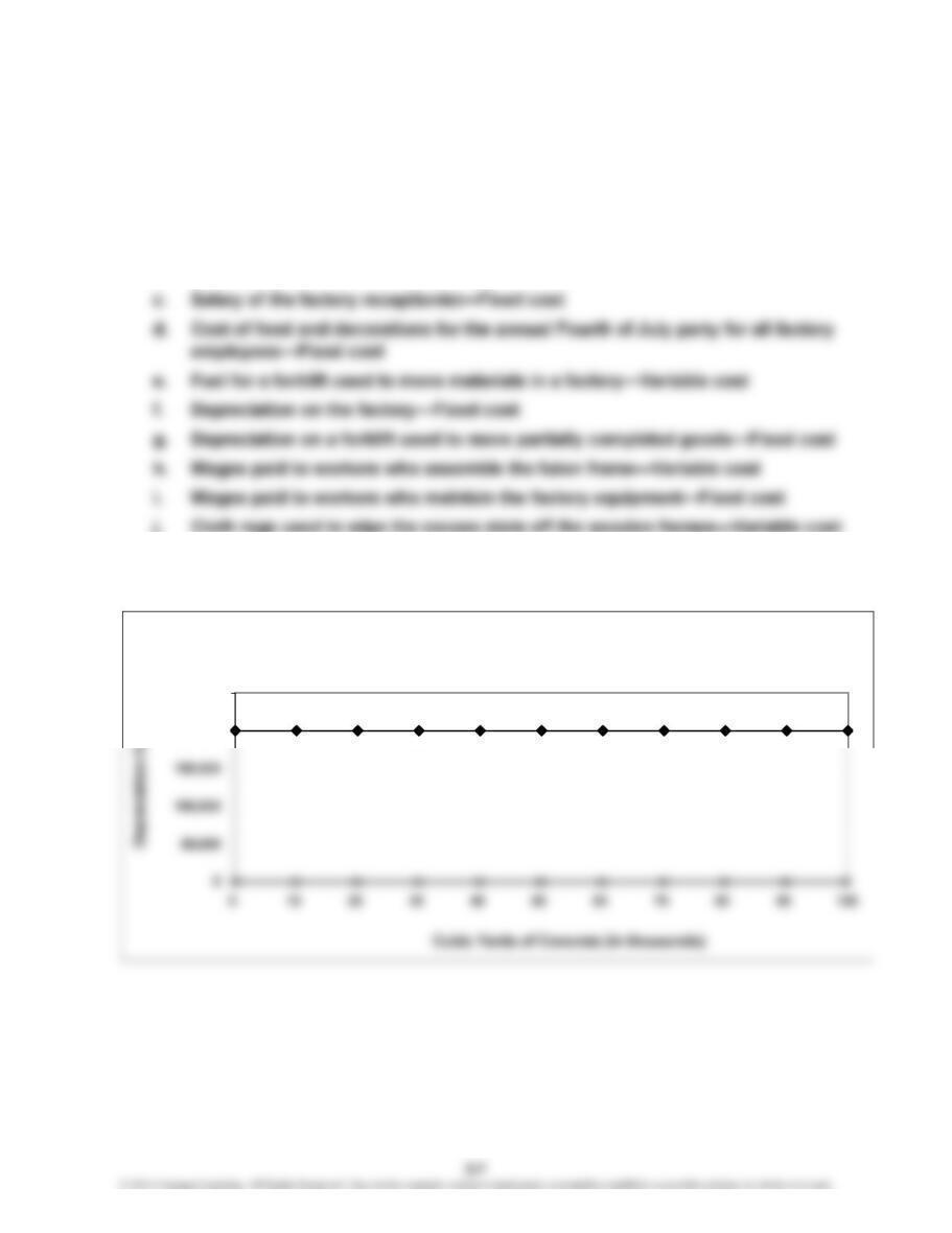
3. Truck depreciation: Fixed cost
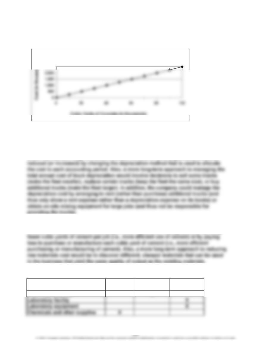
Raw materials cost: Variable cost
4. Truck depreciation is a fixed cost (with respect to the driver “cubic yards of cement”).
Therefore, it cannot be managed by altering the number of cubic yards of cement,
within the relevant range of course. Instead, the cost of truck depreciation could be
5. Raw materials is a variable cost (with respect to the driver “cubic yards of cement”).
Therefore, total raw material cost likely is best reduced (or managed) either by using
E 3-22
Technician salaries
Cost Cate
g
or
y
Variable
Cost
Discretionary
Fixed Cost
Committed
Fixed Cost
X
Raw Materials Cost
2,500
CHAPTER 3 Cost Behavior
E 3-23
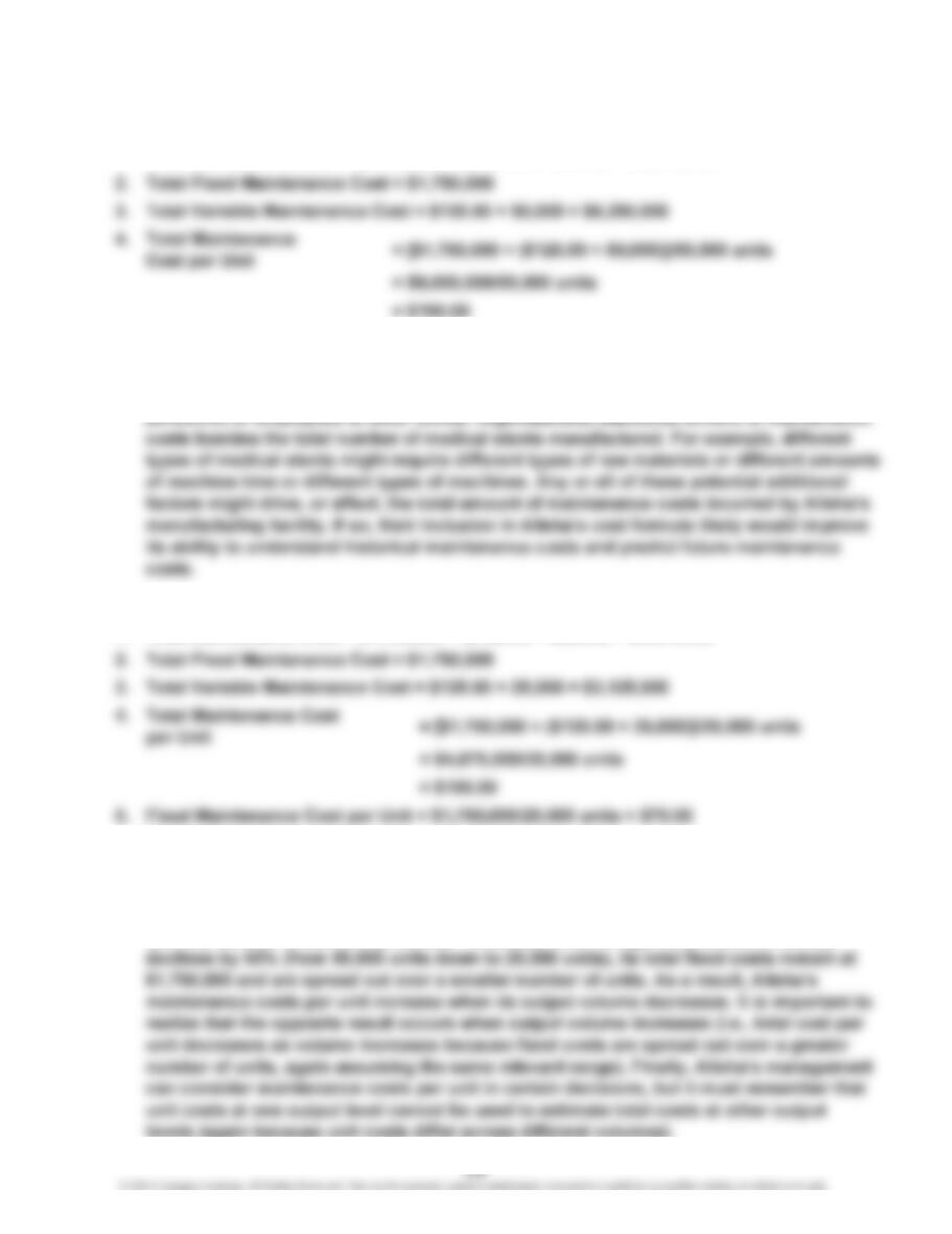
1. Total Maintenance Cost = $1,750,000 + ($125.00 × 50,000) = $8,000,00
0
5. Fixed Maintenance Cost per Unit = $1,750,000/50,000 units = $35.0
0
6.
V
ariable Maintenance Cost per Unit = $125.0
0
7. Alisha management could identify (via research or conversations with its operation
s
E 3-24
1. Total Maintenance Cost = $1,750,000 + ($125.00 × 25,000) = $4,875,00
0
0
6.
V
ariable Maintenance Cost per Unit = $125.0
0
7. The maintenance cost per unit in Exercise 3-24 is higher ($195) than in Exercise 3-2
3
($160) because Alisha incurs fixed costs of $1,750,000 to produce its stents. Assuming
25,000 and 50,000 stents are within the relevant range, Alisha’s fixed costs do not vary
with the number of stents it produces. Therefore, even though its production volume
CHAPTER 3 Cost Behavior
E 3-25
1.
2.
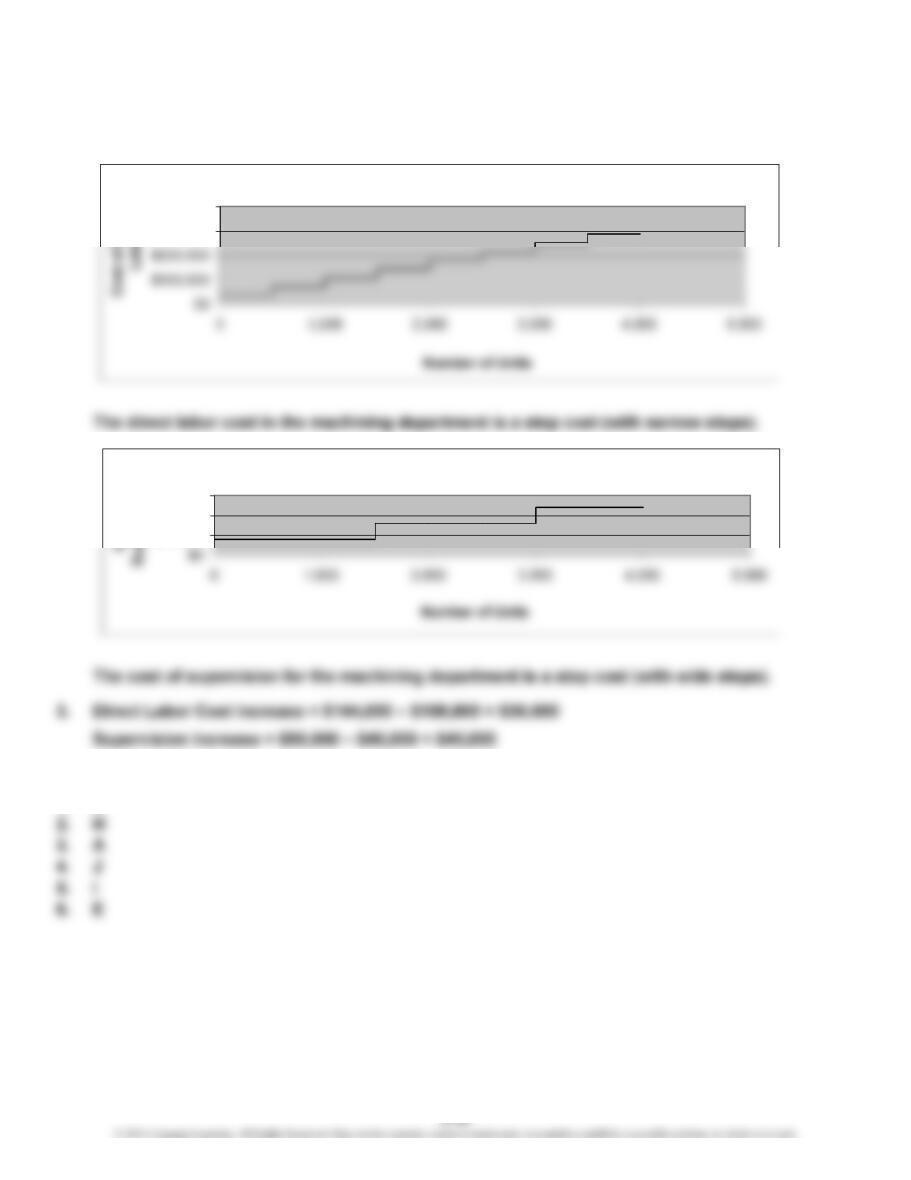
E 3-26
1. K
Direct Labor Cost
$300,000
$400,000
Supervision Cost
$50,000
$100,000
$150,000
CHAPTER 3 Cost Behavior
E 3-27
1. A, B, C (starts off as purely variable and then becomes purely fixed), E, I, and J
Note: The graph in G depicts a situation in which the incremental variable cost per unit
2. H and K
3. D (starts off as purely fixed and then becomes mixed) and F
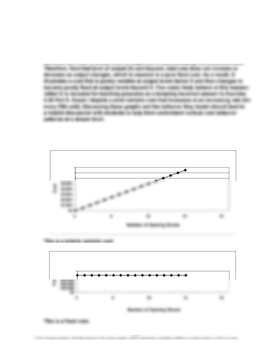
E 3-28
2.
1. Cost of Giving Opening Shows
$6,000
$7,000
$8,000
Cost of Running Gallery
$80,000
$100,000
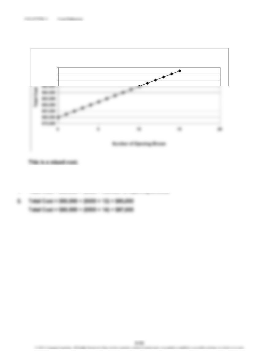
E 3-28 (Continued)
3.
E 3-29
1. Total Cost = $80,000 + ($500 × Number of Opening Shows)
Ben’s Total Costs
$86,000
$87,000
$88,000
E 3-30
1. The high point is March with 3,500 appointments. The low point is May
with 1,500 appointments.
3. Total Tanning Service Cost = $1,040 + ($0.50 × Number of Appointments)
4. Total Predicted Cost for September = $1,040 + ($0.50 × 2,500) = $2,290
5. Using the high-low method means that Luisa’s estimate of the cost formula
(and therefore the cost behavior patterns) is based on only two data points and
ignores all of the other data. She should investigate to be sure that neither the
high nor the low data point are outliers that would distort the cost formula
CHAPTER 3 Cost Behavior
E 3-31
E 3-32
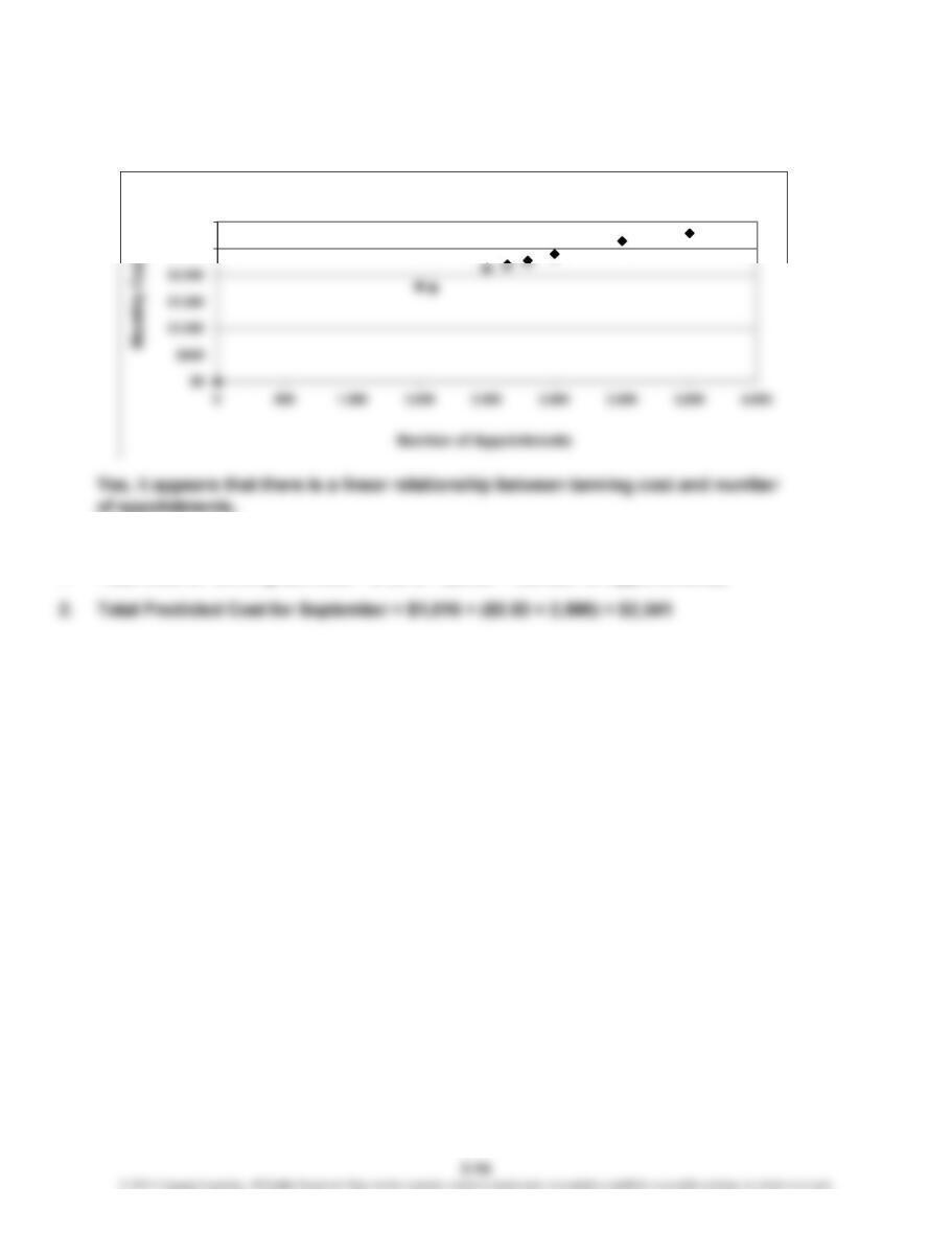
1. Total Cost of Tanning Services = $1,016 + ($0.53 × Number of Appointments)
Scattergraph of Tanning Services
$2,500
$3,000
CHAPTER 3 Cost Behavior
E 3-33
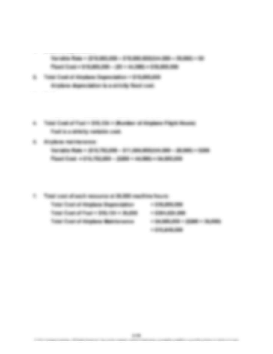
1. Airplane depreciation:
3. Fuel:
Variable Rate = ($445,896,000 – $283,752,000)/(44,000 – 28,000) = $10,134
Fixed Cost = $445,896,000 – ($10,134 × 44,000) = $0
6. Total cost of airplane maintenance:
$4,000,000 + ($268 × Number of Airplane Flight Hours)
Airplane maintenance is a mixed cost.
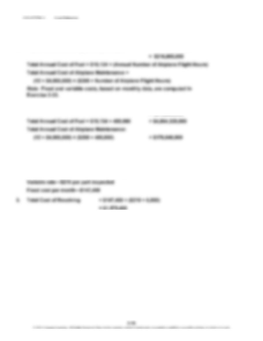
E 3-34
1. Total Annual Cost of Airplane Depreciation = 12 × $18,000,000
2. Total Annual Cost of Airplane Depreciation = 12 × $18,000,000
= $216,000,000
E 3-35
1. Total Cost of Receiving = $147,400 + ($210 × Number of Parts Inspected)
2. Independent variable—number of parts inspected
Dependent variable—total cost of receiving
CHAPTER 3 Cost Behavior
E 3-36
1. Total Annual Cost of Receiving:
E 3-37
1. Overhead cost……………
…
Dependent variable
$150,000…………………… Fixed cost (intercept)
$52…………………………
…
Variable rate (slope)
CHAPTER 3 Cost Behavior
E 3-38
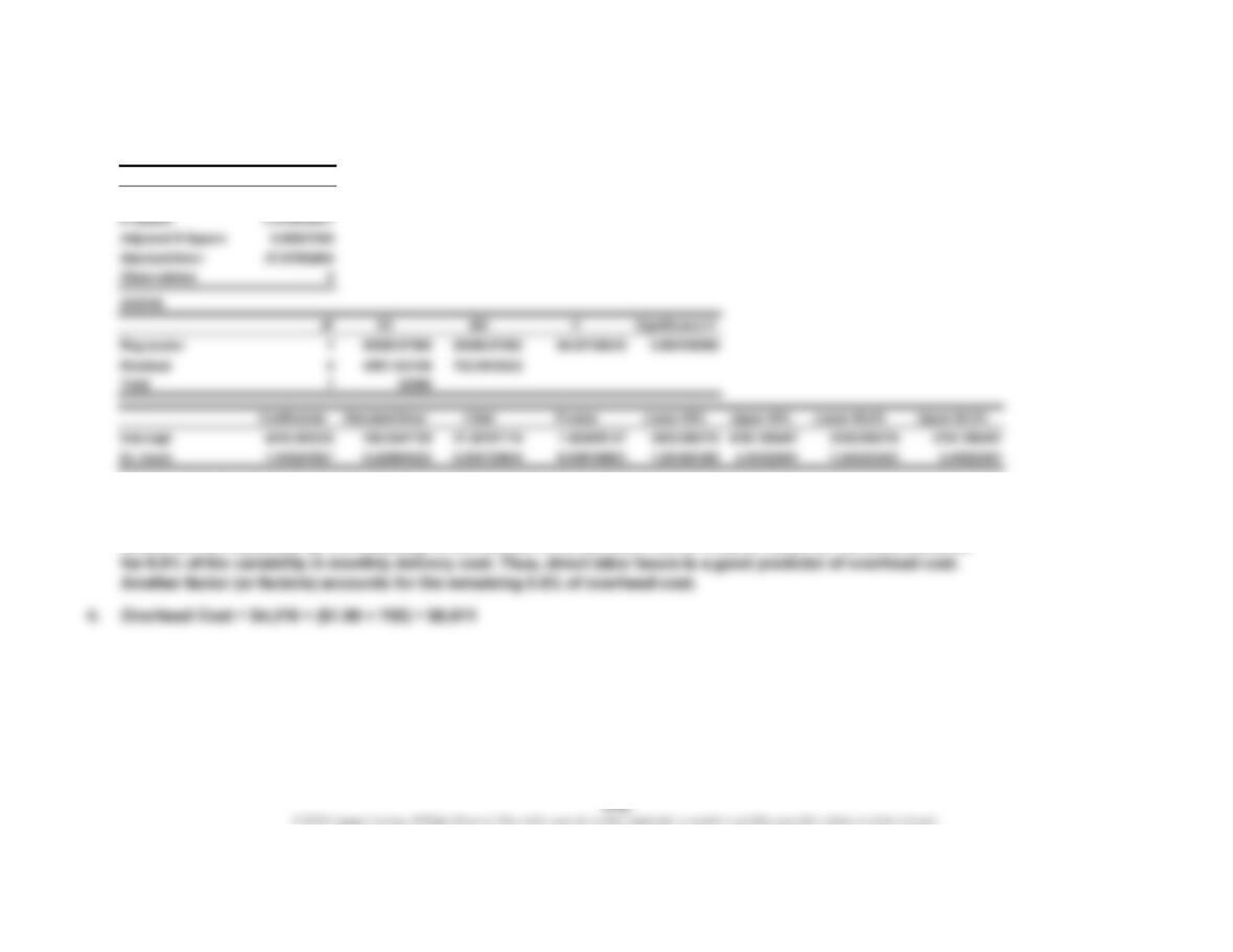
1. SUMMARY OUTPUT
Multiple R 0.95657699
2. Overhead Cost = $4,316 + ($1.85 × Number of Direct Labor Hours)
3. The R² is 0.915, or 9,150.4%. In other words, 91.5% of the variation in the monthly overhead costs from month to
month can be explained by the variability in the number of direct labor hours. Another factor (or factors) accounts
Regression Statistics