CHAPTER 3 Cost Behavior and Forecasting
P 3-64
1. Variable costs—salary of the two paralegals times the percentage of time spent in
processing uncontested claims; salary of the accountant times the percentage of time
spent in this activity; cost of claims forms, checks, envelopes, and postage.
Fixed costs—salaries of the two paralegals times the percentage of time spent in
handling contested claims; depreciation on office equipment used in claims processing
3. The low point is March with $31,260 cost and 4,900 claims; the high point is June with
$44,895 cost and 7,930 claims.
V
ariable Rate = ($44,895 – $31,260)/(7,930 – 4,900)
= $13,635/3,030 claims
= $4.50 per claim
Using the high point:
Fixed Cost = $44,895 – ($4.50 × 7,930) = $9,210
Total Cost of Claims Processing = $9,210 + ($4.50 × Claims)
CHAPTER 3 Cost Behavior and Forecasting
P 3-65
1. The state unemployment insurance premiums and the average cost per injury are fixed
with respect to the number of speakers sold. The state unemployment insurance
premiums are variable (to an extent) with respect to the number of injury claims. That is,
2. Yes, the safety program paid for itself. There was a $50,000 reduction in annual cost of
state unemployment insurance premiums and a $22,000 reduction in the total cost of
injuries per year [$22,500 ($1,500 × 15) – $500 ($50 × 10)]. This is a monetary reduction
CHAPTER 3 Cost Behavior and Forecasting
P 3-66
1. Direct materials……………………….………………
…
$2.85
Direct labor……………………….……………………
…
1.92
V
ariable overhead……………………….……………
…
1.60
2. Absorption-costing income:
Sales (204,300 units × $9)…….………….……………….………….
…
$1,838,700
Less: Cost of goods sold (204,300 units × $7.27)………………… 1,485,261
Gross margin………………………………………………………… $ 353,439
Less: Selling and administrative expenses……………………….
…
279,870
Operating income…………………………………….……………
…
$ 73,569
3. Direct materials……………………….………………
…
$2.85
Direct labor……………………….……………………
…
1.92
V
ariable overhead……………………….……………
…
1.60
Total……………………….…………………………
…
$6.37
Per-unit inventory cost under variable costing equals $6.37.
4.
V
ariable-costing income:
Sales (204,300 units × $9)…….………….……………….………….
…
$1,838,700
Less variable expenses:
V
ariable cost of goods sold (204,300 units × $6.37)…………
…
1,301,391
V
ariable selling and administrative (204,300 units × $0.90)… 183,870
Contribution margin……………………………………………………
…
$ 353,439
Less fixed expenses:
…
…
CHAPTER 3 Cost Behavior and Forecasting
P 3-66 (Continued)
5. Absorption-costing income:
Sales (196,700 units × $9)……………………………………………… $1,770,300
Less: Cost of goods sold (196,700 units × $7.27)…………………
…
1,430,009
V
ariable-costing income:
Sales (196,700 units × $9)……………………………………………… $1,770,300
Less variable expenses:
V
ariable cost of goods sold (196,700 units × $6.37)……………… 1,252,979
V
ariable selling and administrative (196,700 units × $0.90)……
…
177,030
Contribution margin………………………………….……………………
…
$ 340,291
…
…
CHAPTER 3 Cost Behavior and Forecasting
P 3-67
1. Results of regressions:
10 Months’ 12 Months’
Data Data
Intercept…………………
…
3,212 3,820
Slope………………………
…
15.15 15.10
R²…………………………
…
0.85 0.75
2.
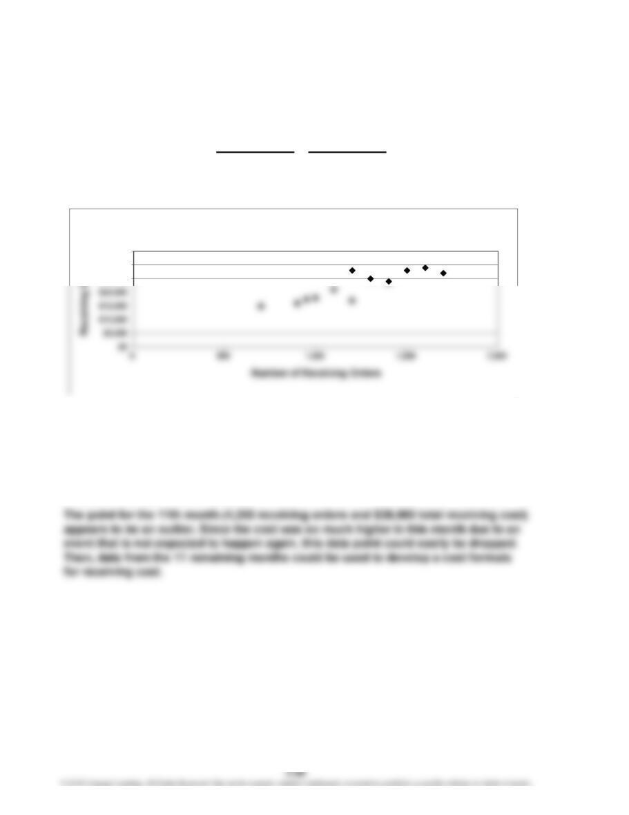
The regression run on the 11 months of data from “typical” months appears to be better
than the one for all 12 months. R² is higher for the regression without the outlier
(85.88% versus 74.51%), and the scattergraph gives Tracy confidence that the data
without the outlier describe a relatively linear relationship. Since the storm damage
is not expected to recur, Month 11 can safely be dropped from a regression meant to
help predict future receiving cost.
$25,000
$30,000
$35,000
Scattergraph of Receiving Activity—12 Month’s Data
CHAPTER 3 Cost Behavior and Forecasting
P 3-67 (Concluded)
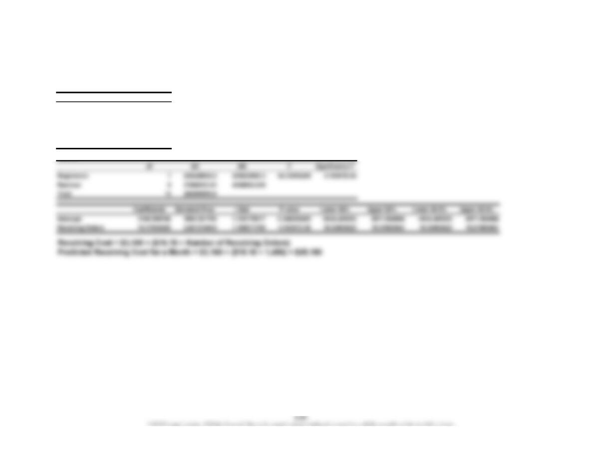
3. Results for the method of least squares after dropping Month 11.
SUMMARY OUTPUT
Regression Statistics
Multiple R 0.926737002
R Square 0.85884147
Adjusted R Square 0.843157189
Standard Error 2051.780599
Observations 11
ANOVA
CHAPTER 3 Cost Behavior and Forecasting
P 3-68
1.
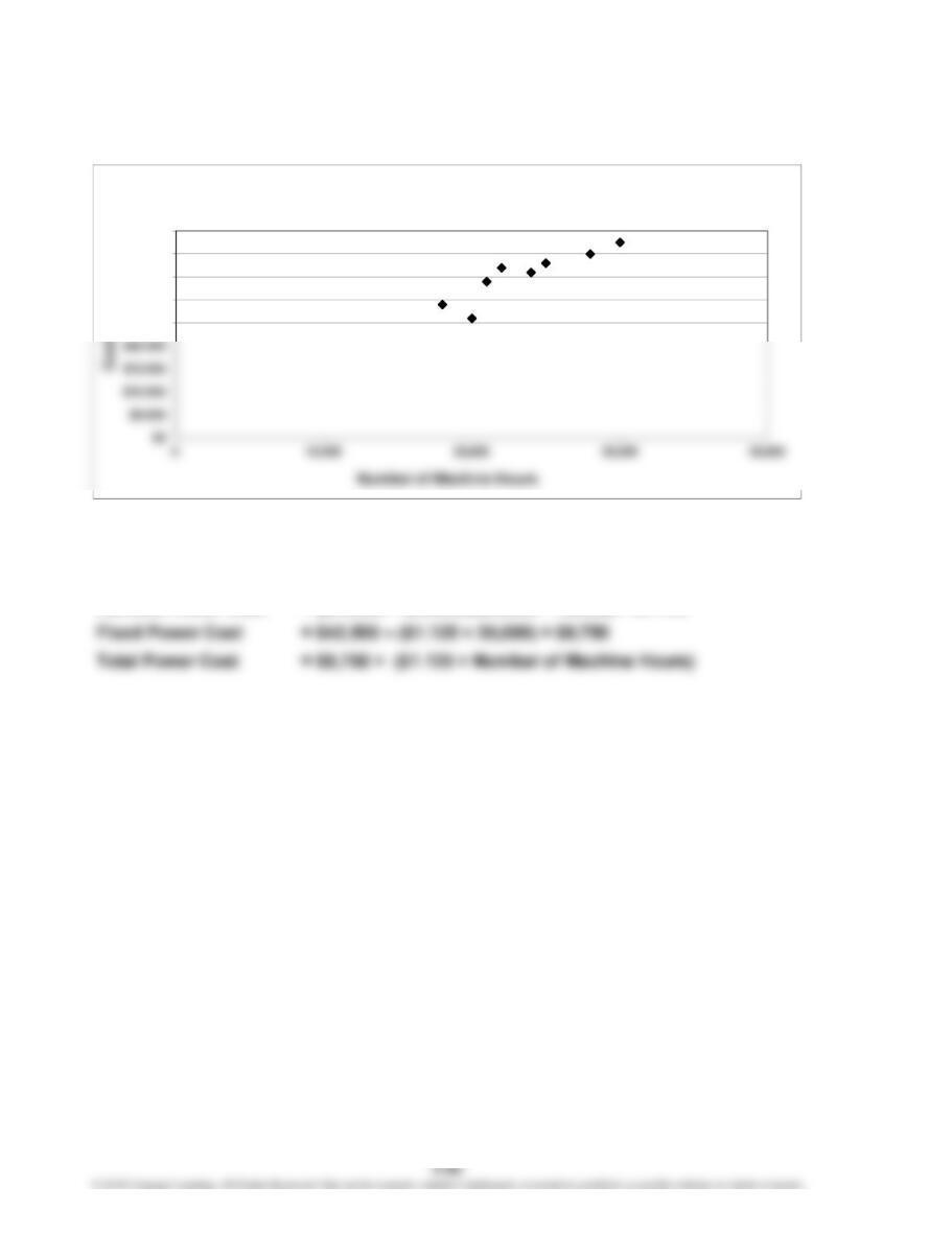
The overall relationship looks reasonably linear—although the data point for the first
quarter may be an outlier.
2. Using the high-low method:
$25,000
$30,000
$35,000
$40,000
$45,000
Scattergraph of Power Cost
CHAPTER 3 Cost Behavior and Forecasting
P 3-68 (Continued)
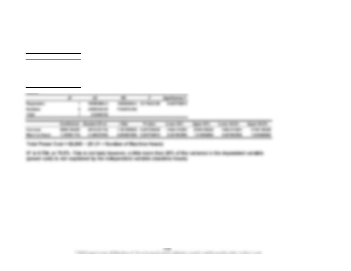
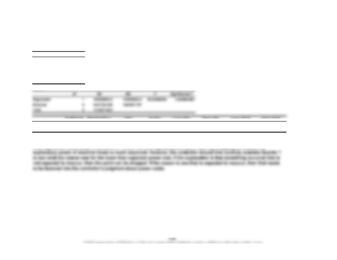
3. Output of regression program:
SUMMARY OUTPUT
Regression Statistics
Multiple R 0.893359672
R Square 0.798091504
Adjusted R Square 0.764440088
Standard Error 2673.924883
Observations 8
CHAPTER 3 Cost Behavior and Forecasting
P 3-68 (Concluded)
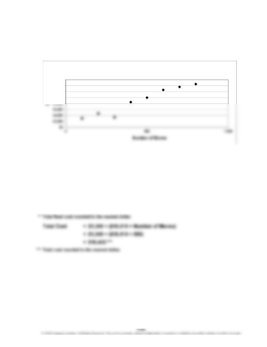
4. The output of a regression program after Quarter 1 (20,000, $26,000) has been dropped.
SUMMARY OUTPUT
Regression Statistics
Multiple R 0.957883502
R Square 0.917540803
Adjusted R Square 0.901048964
Standard Error 1367.284823
Observations 7
Coefficients Standard Error t Stat P-value Lower 95% Upper 95% Lower 95.0% Upper 95.0%
Intercept 12407.56303 3289.994132 3.771302479 0.013005506 3950.363873 20864.76218 3950.363873 20864.76218
Machine Hours 1.009803922 0.135381371 7.458957725 0.000683462 0.661795029 1.357812814 0.661795029 1.357812814
Total Power Cost = $12,408 + ($1.01 × Number of Machine Hours)
CHAPTER 3 Cost Behavior and Forecasting
P 3-69
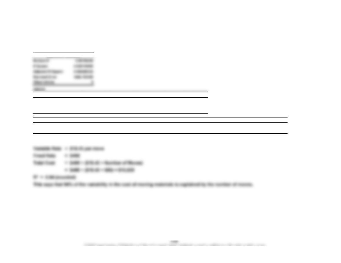
1. The scattergraph provides evidence for a linear relationship, but the observation for
300 moves may be an outlier.
2. High (800, $14,560); Low (100, $3,000)
V
ariable Rate = ($14,560 – $3,000)/(800 – 100)
= $11,560/700 moves
= $16.514
*Variable rate rounded to three decimal places.
Fixed Rate Cost = $3,000 – ($16.514 × 100)
= $3,000 – $1,651.40
= $1,349
$10,000
$12,000
$14,000
$16,000
Cost of Moving Materials
*
**
CHAPTER 3 Cost Behavior and Forecasting
P 3-69 (Continued)
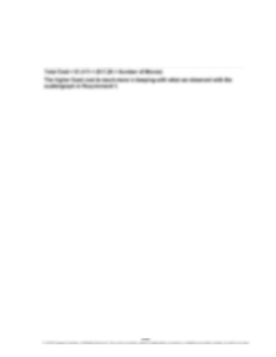
3. Output of the regression routine calculated by a spreadsheet:
SUMMARY OUTPUT
df SS MS F Significance F
Regression 1 142581862.5 142581862.5 88.86165795 8.10236E-05
Residual 6 9627225 1604537.5
Total 7 152209087.5
Coefficients Standard Error t Stat P-value Lower 95% Upper 95% Lower 95.0% Upper 95.0%
Intercept 497.5 987.0073364 0.504048938 0.63219637 -1917.619944 2912.619944 -1917.619944 2912.619944
Number of Moves 18.425 1.954565778 9.426646167 8.10236E-05 13.64234984 23.20765016 13.64234984 23.20765016
Rounding the coefficients:
CHAPTER 3 Cost Behavior and Forecasting
P 3-69 (Concluded)
4. Normally, we would prefer the least squares method since the data appear to be linear.
However, the third observation may be an outlier. If the third observation (300 moves
and $3,400 of cost) is dropped, the R² rises to 99%. The new cost formula would be:
CHAPTER 3 Cost Behavior and Forecasting
Case 3-70
1. The order should cover the variable costs described in the cost formulas.
These variable costs represent flexible resources.
Materials ($94 × 20,000)……………………………………………………
…
$1,880,000
Labor ($16 × 20,000)…………………………………………………………
…
320,000
V
…
V
…
2. The coefficients of determination indicate the reliability of the cost formulas.
Of the four formulas, overhead activity may be a problem. A coefficient of
determination of 0.56 means that only about 56% of the variability of
3. Resource spending attributable to order:
Materials ($94 × 20,000)…………………………………………….………
…
$1,880,000
Labor ($16 × 20,000)…….…………………………………….…..…………
…
320,000
V
ariable overhead:
($85 × 20,000)……………….……………………………….……………
…
1,700,000
($5,000 × 12)…………………………….…………………………………
…
60,000
V
…
…
CASES
Case 3-70 (Concluded)
It would also be useful to know the step-cost functions for any activities that have
resources acquired in advance of usage on a short-term basis. It is possible that
Case 3-71
1. Carl’s behavior is definitely unethical. He is stealing confidential information from
Kilborn and using it for unethical advantages. Kilborn would not approve of Carl’s
actions and would have a potential lawsuit against him for theft of information.
2. Assuming that the data were acquired illicitly, Bill’s instincts were on target. To hire
Carl in implicit exchange for the confidential information would be a violation of