Problem 3.35 (Concluded)
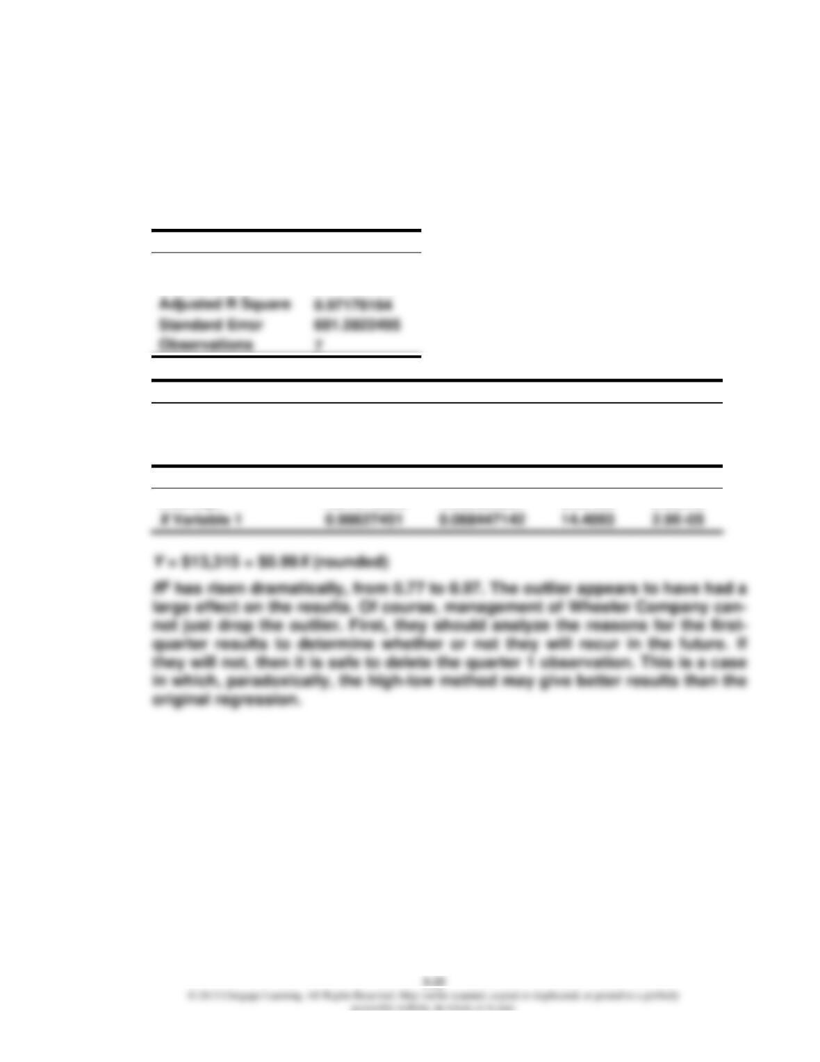
4. Regression output from spreadsheet, leaving out the first quarter observation
(20,000, $26,000), which appears to be an outlier:
SUMMARY OUTPUT
Regression Statistics
Multiple R
0.98817240
R Square
0.97648470
Adjusted R Square
0.97178164
Standard Error
691.2822495
Observations
7
ANOVA
df
SS
MS
F
Regression
1
99219215.69
9.9E+07
207.628
Residual
5
2389355.742
477871
Total
6
101608571.4
Coefficients
Standard Error
t Stat
P-value
Intercept
13315.12605
1663.380231
8.00486
0.00049
Problem 3.36
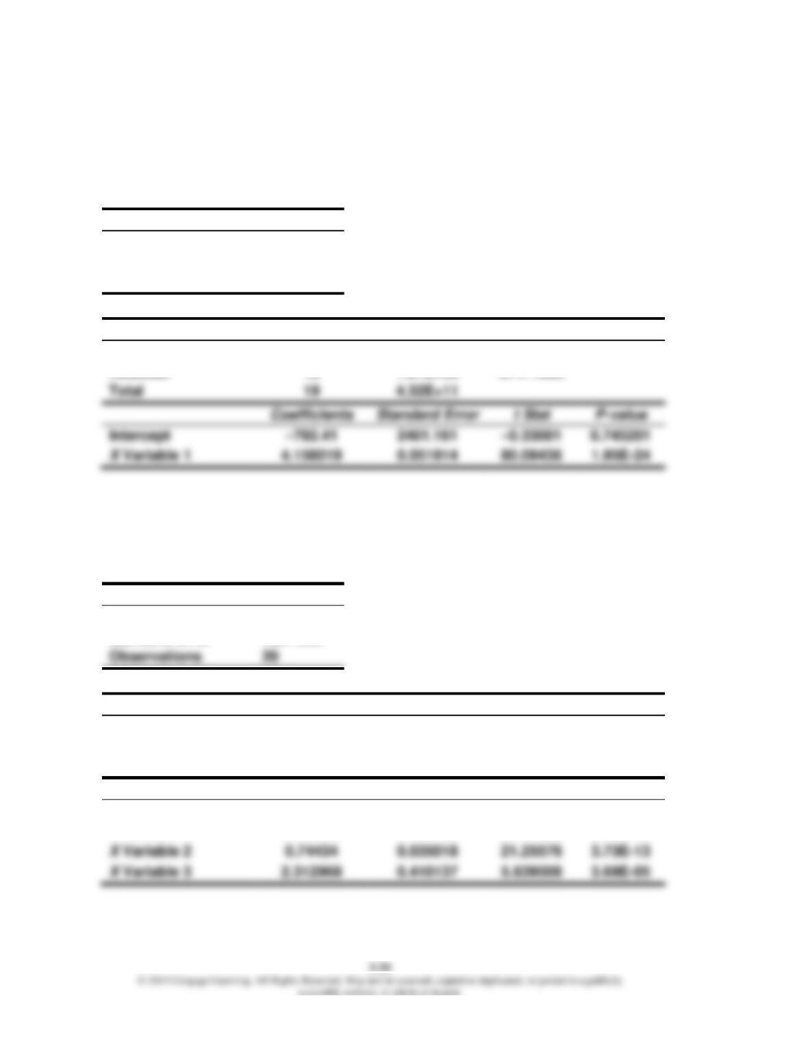
1. Regression output from spreadsheet for X = number of orders:
SUMMARY OUTPUT
Regression Statistics
Adjusted R Square
0.997047
Standard Error
8195.827
Observations
20
ANOVA
df
SS
MS
F
Regression
1
4.31E+11
4.31E+11
6415.107
Residual
18
1.21E+09
67171580
Total
Coefficients
Standard Error
t Stat
P-value
Intercept
2401.161
0.745201
2. Multiple regression output from spreadsheet for X1 = number of orders, X2 =
weight in pounds; X3 = number of fragile orders:
SUMMARY OUTPUT
Regression Statistics
Adjusted R Square
0.999886
Standard Error
1607.632
Observations
ANOVA
df
SS
MS
F
Regression
3
4.32E+11
1.44E+11
55727.57
Residual
16
41351702
2584481
Total
19
4.32E+11
Coefficients
Standard Error
t Stat
P-value
Intercept
474.7219
475.7715
0.997794
0.333231
X Variable 1
2.100464
0.104728
20.05633
9.16E-13
Problem 3.36 (Concluded)
The first regression equation has a very high R2; however, fixed cost is nega-
tive (but not significant) and the standard error is large. The multiple regres-
sion equation is much better. R2 is still very high (0.99), but all three variables
are significant. The fixed cost, while still not significant, is positive, and the
standard error is much smaller.
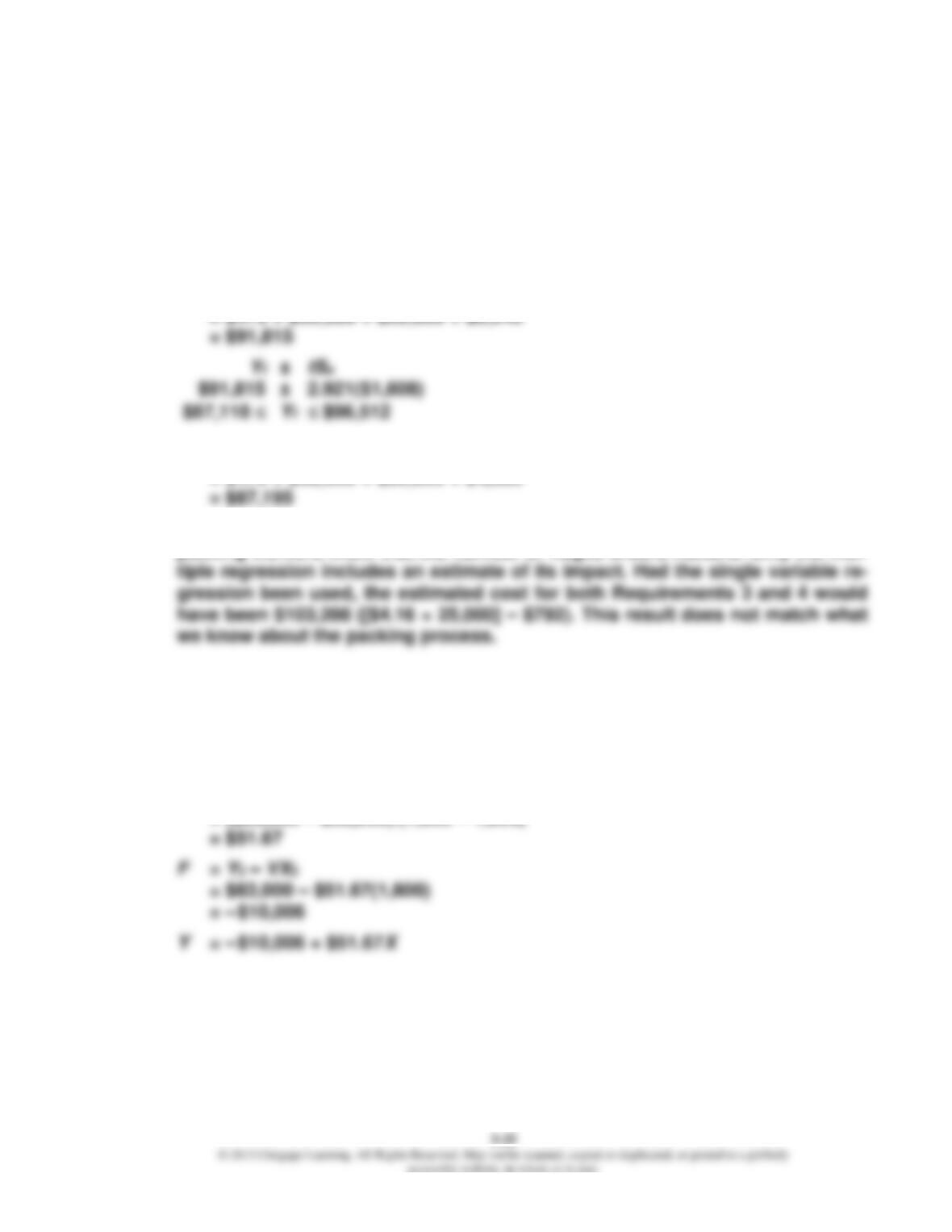
3. Y = $475 + $2.10(25,000) + $0.74(40,000) + $2.31(4,000)
= $475 + $52,500 + $29,600 + $9,240
4. Y = $475 + $2.10(25,000) + $0.74(40,000) + $2.31(2,000)
= $475 + $52,500 + $29,600 + $4,620
This result gives us more confidence in using the multiple regression. The
packing workers know that the number of fragile orders matters. Only the mul-
Problem 3.37
1. High: 1,800, $83,000
Low: 1,200, $52,000
V = (Y2 – Y1)/(X2 – X1)
= ($83,000 – $52,000)/(1,800 – 1,200)
Problem 3.37 (Continued)
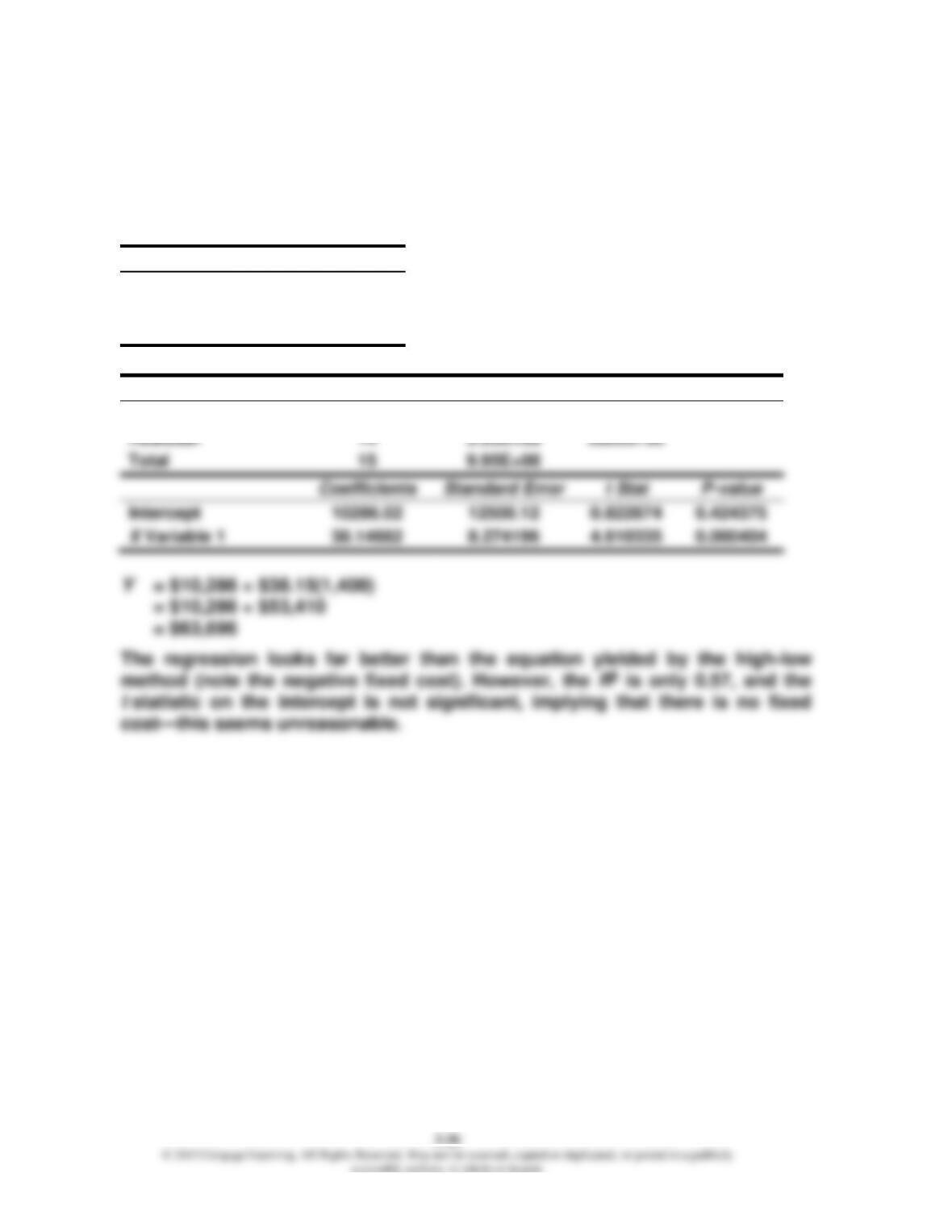
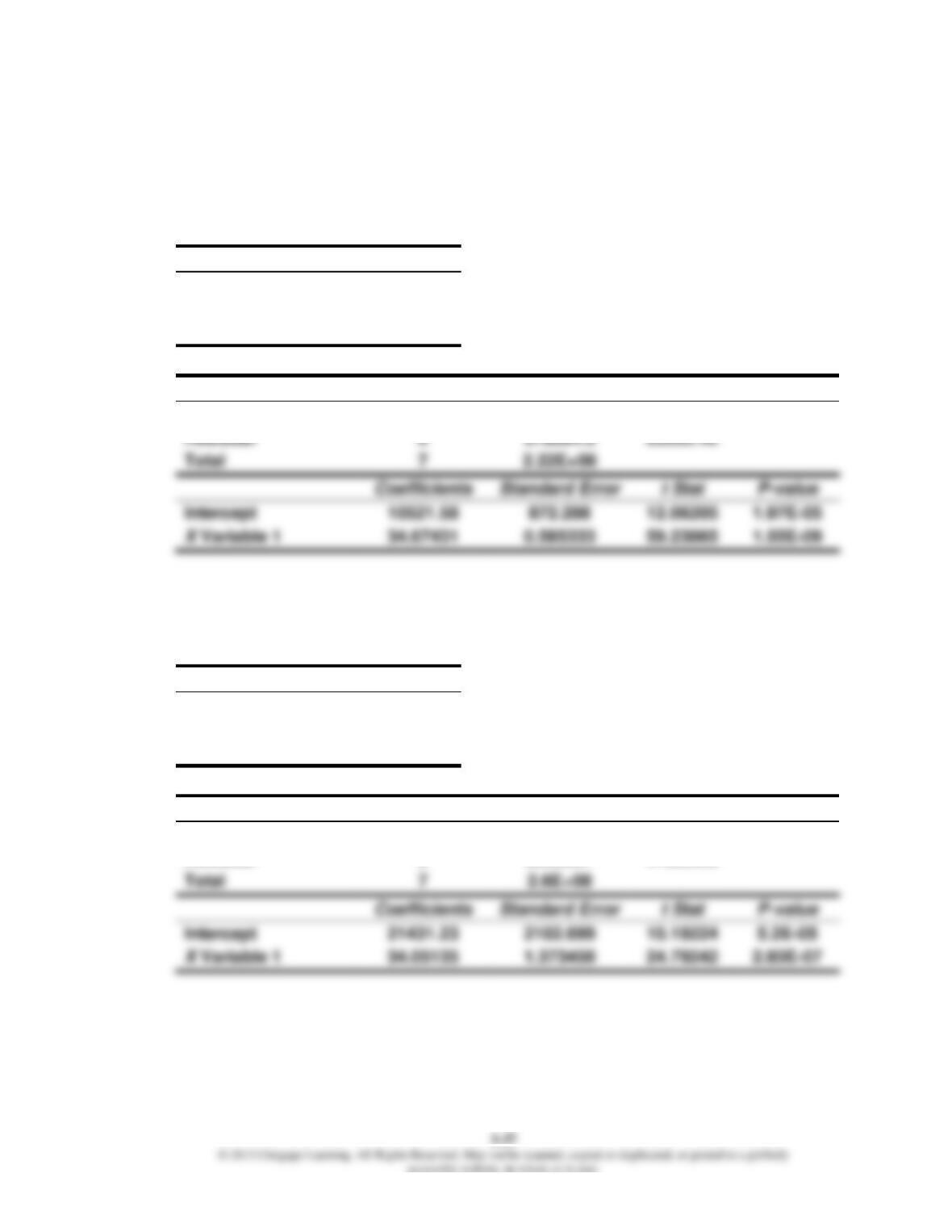
2. Regression output from spreadsheet:
SUMMARY OUTPUT
Regression Statistics
Adjusted R Square
0.574531
Standard Error
5311.289
Observations
16
ANOVA
df
SS
MS
F
Regression
1
6E+08
6E+08
21.25519
Total
Intercept
0.822874
0.424375
Problem 3.37 (Continued)
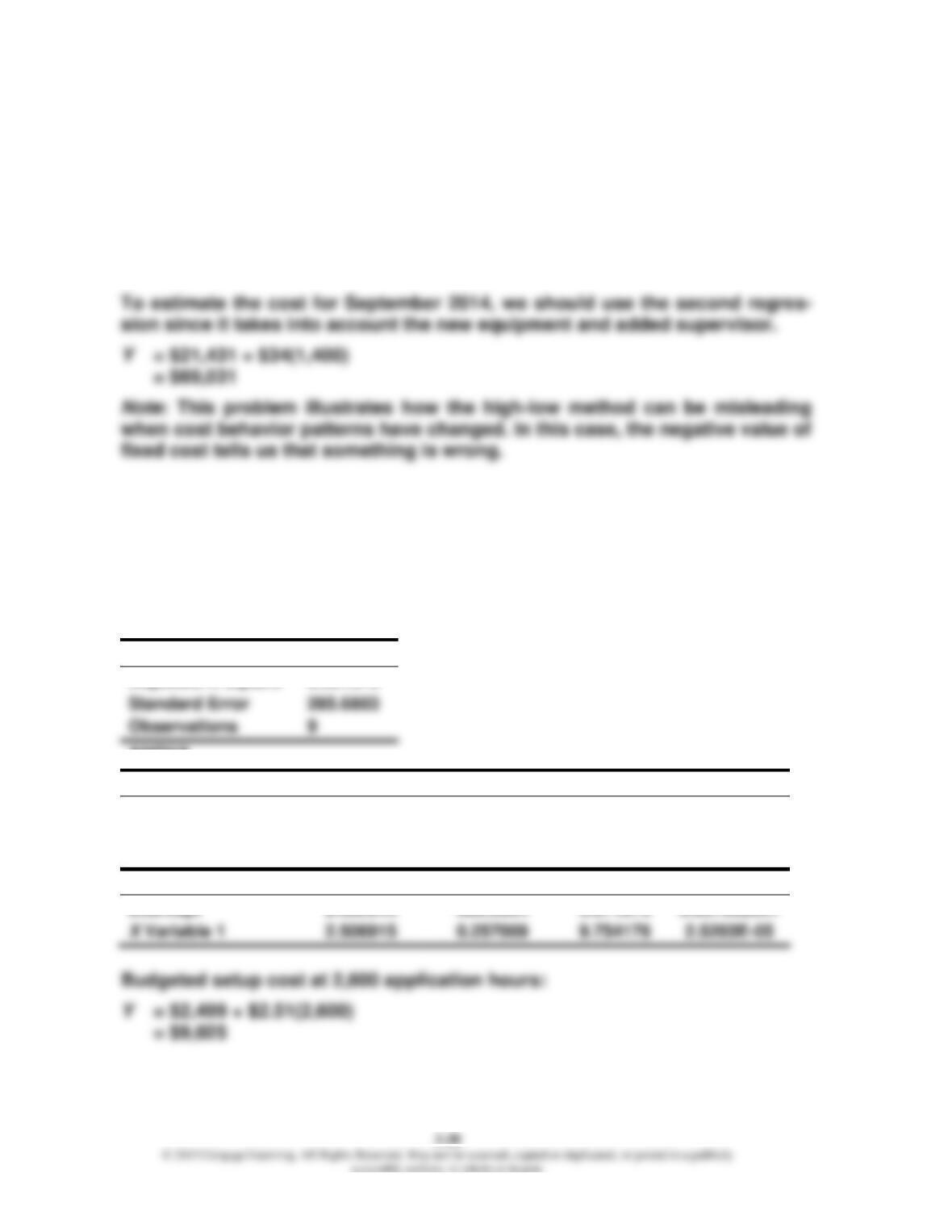
3. Regression output from the spreadsheet for the first eight observations:
SUMMARY OUTPUT
Regression Statistics
Adjusted R Square
0.998009
Standard Error
251.182
Observations
8
ANOVA
df
SS
MS
F
Regression
1
2.21E+08
2.21E+08
3509.218
Residual
6
63092.42
Total
Intercept
12.06205
Regression output from the spreadsheet for the last eight observations:
SUMMARY OUTPUT
Regression Statistics
Adjusted R Square
0.988722
Standard Error
646.6887
Observations
8
ANOVA
df
SS
MS
F
Regression
1
2.57E+08
2.57E+08
614.664
Residual
6
2509237
418206.2
Total
Intercept
10.19224
Problem 3.37 (Concluded)
The results from these two regressions are far more reasonable! We can see
the nearly $10,000 shift upward in fixed cost from the first intercept to the sec-
ond. The R2 for both regressions is 0.99, and in both regressions, the fixed
cost and variable rate are significant, as measured by the t statistics. Finally,
the standard errors are much smaller than the one in the regression in Re-
quirement 2.
Problem 3.38
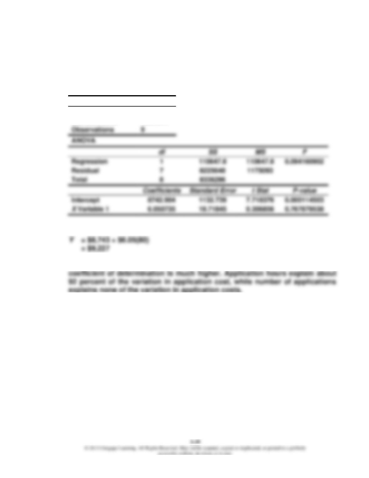
1. Regression output from spreadsheet, application hours as X variable:
SUMMARY OUTPUT
Regression Statistics
Adjusted R Square
0.921679
Observations
9
ANOVA
df
SS
MS
F
Regression
1
7765004
7765004
95.14395498
Residual
7
571292.5
81613.21
Total
8
8336296
Coefficients
Standard Error
t Stat
P-value
Intercept
2498.644
680.6304
3.671073
0.007952951
Problem 3.38 (Continued)
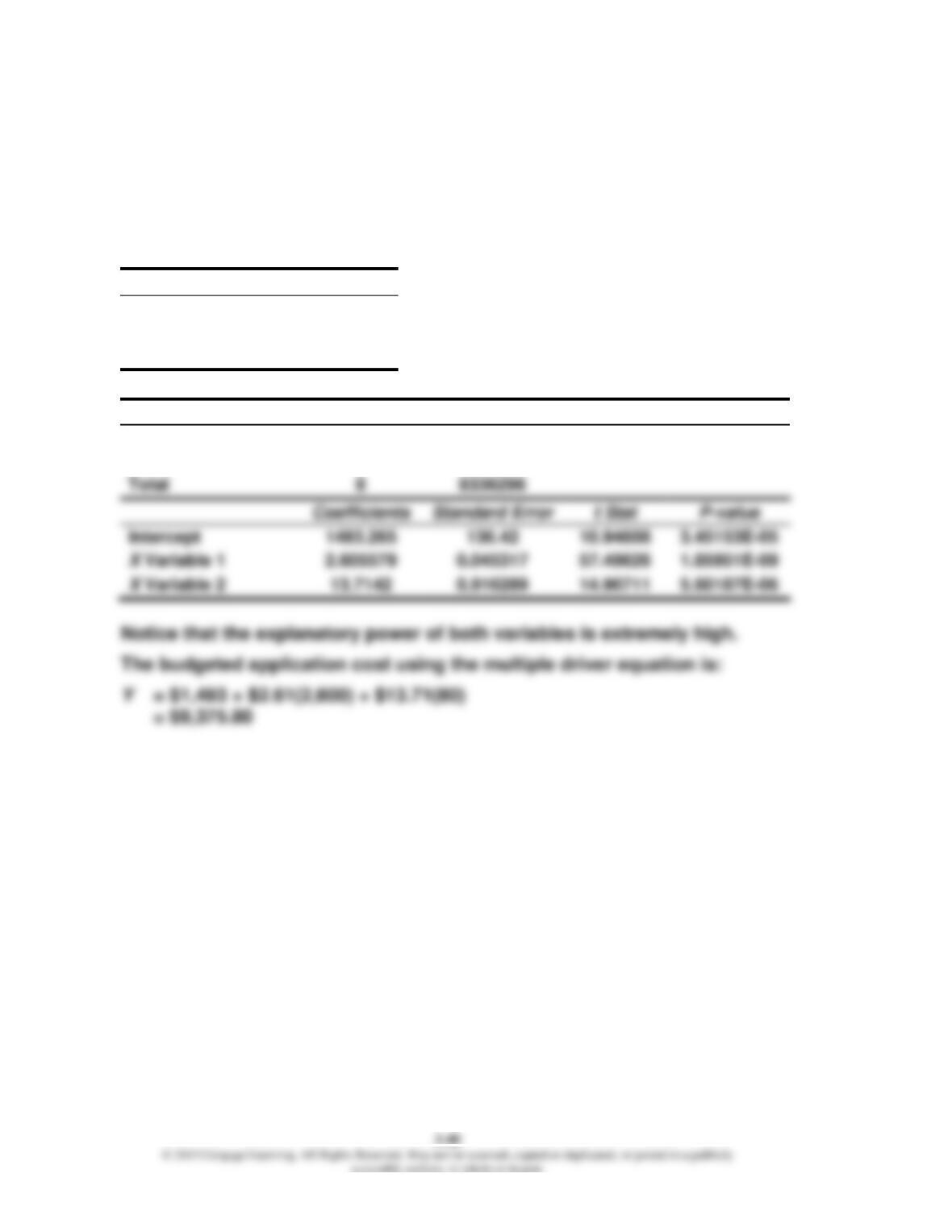
2. Regression output from spreadsheet, number of applications as X variable:
SUMMARY OUTPUT
Regression Statistics
Adjusted R Square
–0.12769
Standard Error
1084.017
9
ANOVA
Total
Budgeted setup costs for 80 applications:
3. The regression equation based on application hours is better because the
Problem 3.38 (Concluded)
4. Regression output from spreadsheet, application hours as X1 variable, num-
ber of applications as X2 variable:
SUMMARY OUTPUT
Regression Statistics
Adjusted R Square
0.997616
Standard Error
49.83698
Observations
9
ANOVA
df
SS
MS
F
Regression
2
8321394
4160697
1675.18476
Residual
6
14902.34
2483.724
Total
Intercept
10.94608
Problem 3.39
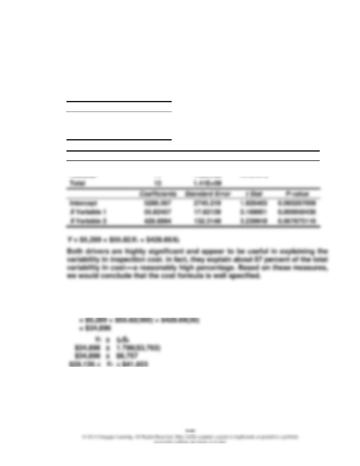
1. Regression output from spreadsheet, inspection hours as X1 variable, num-
ber of batches as X2 variable:
SUMMARY OUTPUT
Regression Statistics
Adjusted R Square
0.869143
Standard Error
3761.810
Observations
14
ANOVA
df
SS
MS
F
Regression
2
1.25E+09
6.25E+08
44.1724979
Residual
1.56E+08
Total
Intercept
1.926465
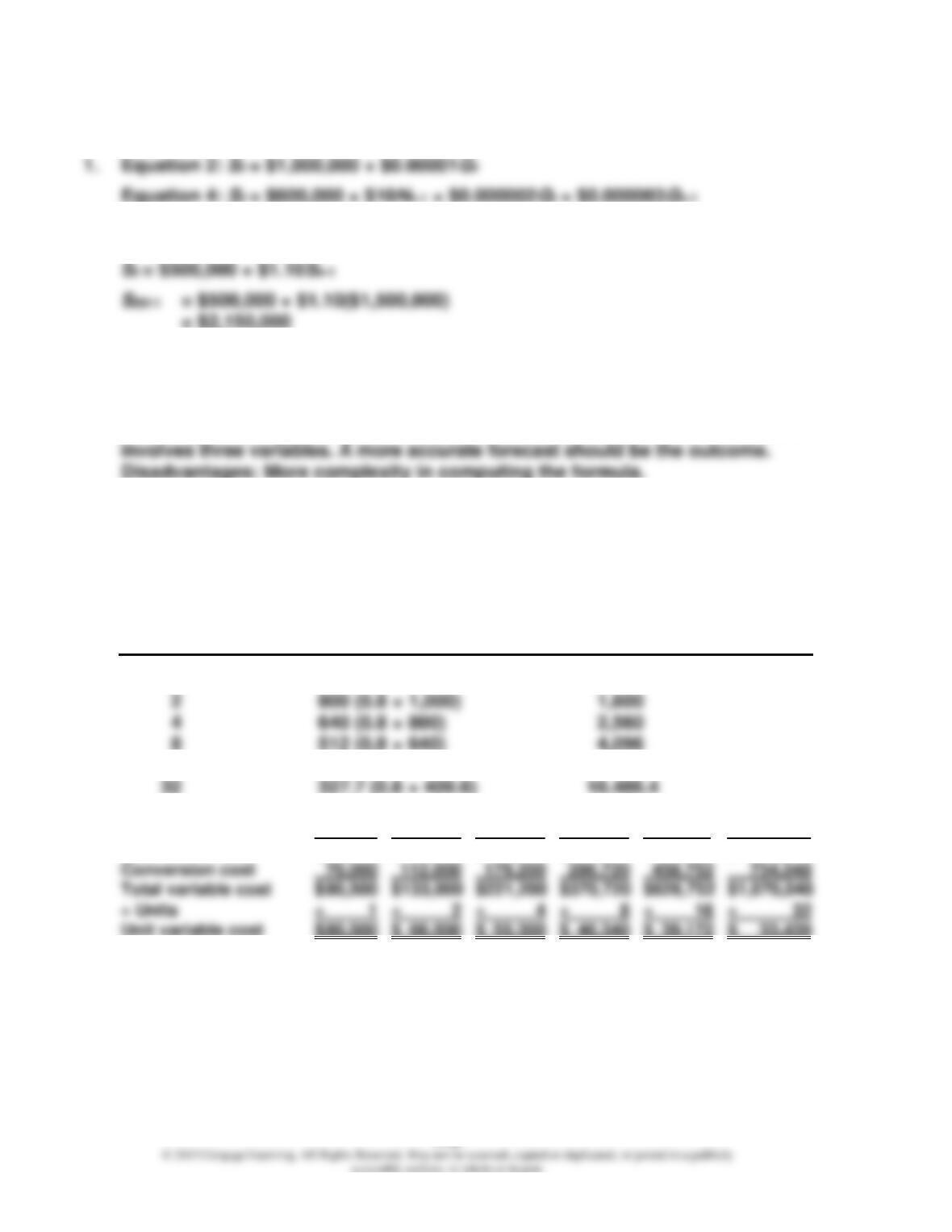
2. When X1 = 300 hours and X2 = 30 batches, we have the following predicted
cost:
Y = $5,289 + $55.82X1 + $428.69X2
3-42
Problem 3.40
2. To forecast 2014 sales based on 2013 sales, Equation 1 must be used:
3. Equation 2 requires a forecast of gross domestic product. Equation 3 uses the
actual gross domestic product for the past year and, therefore, is observable.
4. Advantages: Using the highest R2, the lowest standard error, and the equation
Problem 3.41
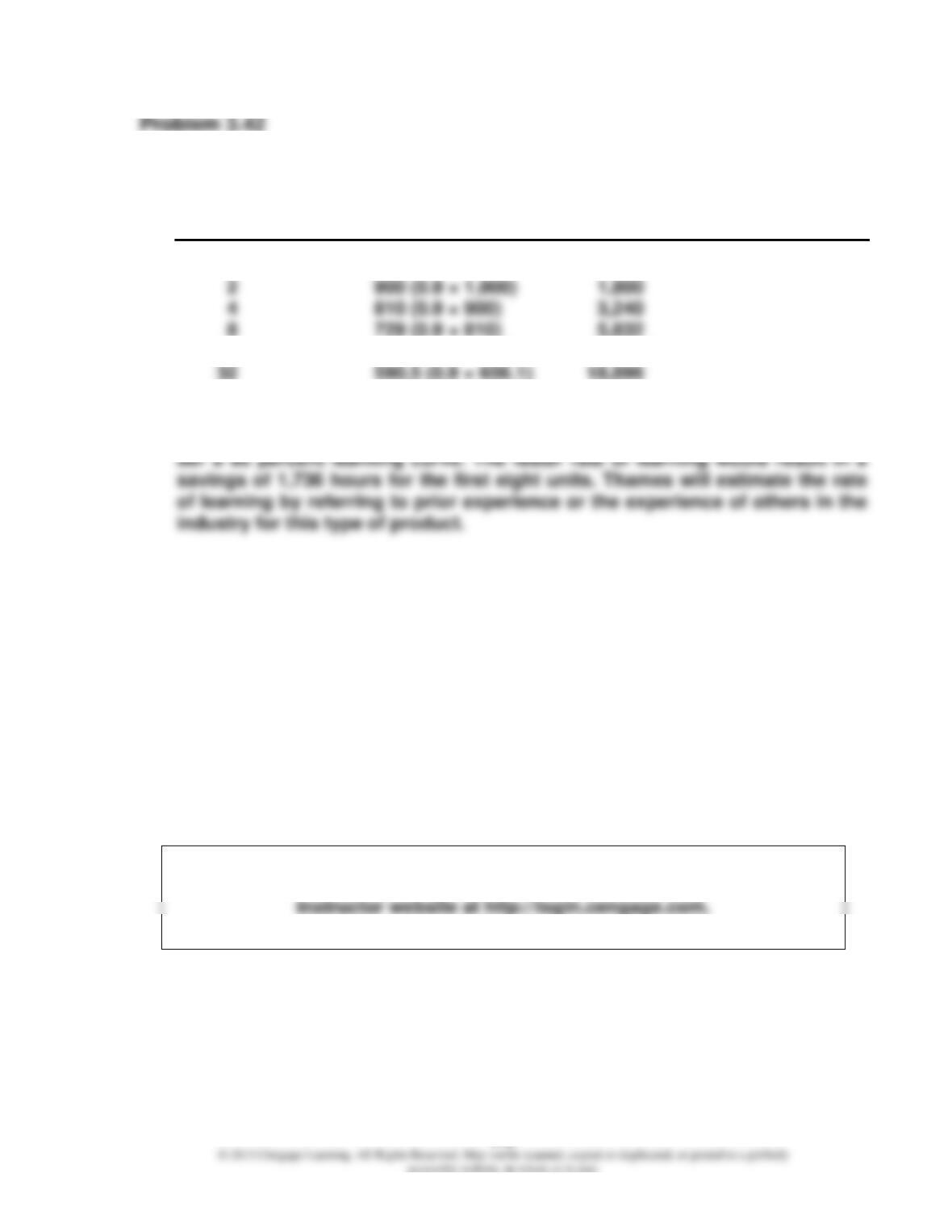
1. Cumulative Cumulative Cumulative
Number Average Time Total Time:
of Units per Unit in Hours Labor Hours
(1) (2) (3) = (1) × (2)
1 1,000 1,000
16 409.6 (0.8 × 512) 6,553.6
2. 1 unit 2 units 4 units 8 units 16 units 32 units
Direct materials $ 10,500 $ 21,000 $ 42,000 $ 84,000 $168,000 $ 336,000
3-43
1. Cumulative Cumulative Cumulative
Number Average Time Total Time:
of Units per Unit in Hours Labor Hours
(1) (2) (3) = (1) × (2)
1 1,000 1,000
16 656.1 (0.9 × 729) 10,497.6
2. If Thames could realize an 80 percent learning curve, the eight units would
take 4,096 hours to sell and service as compared to the 5,832 estimated un-
CYBER RESEARCH CASE
3.43
Answers will vary.
The Collaborative Learning Exercise Solutions can be found on the
3-44
The following problems can be assigned within CengageNOW and are auto-
graded. See the last page of each chapter for descriptions of these new assign-
ments.
• Analyzing Relationships—Practice altering the Total Fixed Costs and the Vari-
able Rate to determine total cost. Setting up Cost-Behavior Based Income
statements.
• Integrative Problem—Cost Behavior, Process Costing, Standard Costing (Cov-
ering chapters 3, 6, and 9)