1. Knowledge of cost behavior allows a manager to assess changes in costs that result from
changes in activity. This allows a manager to examine the effects of choices that change activity.
For example, if excess capacity exists, bids that at least cover variable costs may be totally
appropriate. Knowing what costs are variable and what costs are fixed can help a manager make
better bids and, ultimately, better business decisions.
4. Some account categories are primarily fixed or variable. Even if the cost is mixed, either the fixed
component or the variable component is relatively small. As a result, assigning all of the cost to
either a fixed or variable category is unlikely to result in large errors. For example, depreciation on
property, plant, and equipment is largely fixed. The cost of telephone expense for the sales office,
if it consisted primarily of long-distance calls, could be seen as largely variable (variable with
respect to the number of customers).
5. Committed fixed costs are those incurred for the acquisition of long-term activity capacity and are
not subject to change in the short run. Annual resource expenditure is independent of actual
usage. For example, the cost of a factory building is a committed fixed cost. Discretionary fixed
costs are those incurred for the acquisition of short-term activity capacity, the levels of which can
be altered quickly. In the short run, resource expenditure is also independent of actual activity
usage. Salaries of engineers are an example of such an expenditure.
6. The concept of relevant range is important in dealing with step costs because if the relevant range
is contained completely within one step, the cost behaves as a fixed cost. However, if the relevant
range spans two or more steps, the accountant must be aware of the cost increase as output
goes up within the relevant range.
7. Mixed costs are usually reported in total in the accounting records. How much of the cost is fixed
and how much is variable is unknown and must be estimated.
3COST BEHAVIOR AND
FORECASTING
DISCUSSION QUESTIONS
CHAPTER 3 Cost Behavior and Forecasting
10.
A
scattergraph allows a visual portrayal of the relationship between cost and activity. It
reveals to the investigator whether a relationship may exist and, if so, whether a linear
function can be used to approximate the relationship.
12. Because the scattergraph method is not restricted to the high and low points, it is
possible to select two points that better represent the relationship between activity and
costs, producing a better estimate of fixed and variable costs. The main advantage of the
high-low method is that it removes subjectivity from the choice process. The same line
will be produced by two different people.
A
14. The best-fitting line is the one that is “closest” to the data points. This is usually
measured by the line that has the smallest sum of squared deviations from the individual
data points.
15. The only difference between absorption costing and variable costing is the way in which
fixed overhead costs are assigned. Under variable costing, fixed overhead is a period cost;
under absorption costing, it is a product cost.
16.
A
bsorption-costing income is greater because some of the period’s fixed overhead is placed
in inventory and not recognized as part of cost of goods sold on the absorption-costing
income statement.
CHAPTER 3 Cost Behavior and Forecasting
3-1. c
3-5. a
3-6. d
3-7. c
3-8. d Total Cost = $235,000 + ($75 × 8,000) = $835,000
3-9. b
3-13. b
3-14. b
MULTIPLE-CHOICE QUESTIONS
CHAPTER 3 Cost Behavior and Forecasting
BE 3-16
1. The cost formula takes the following form:
Total Cost = Fixed Cost + (Variable Rate × Number of Flash Drives)
The monthly fixed cost is the $15,000 cost of equipment depreciation, as it does not
vary according to the number of flash drives manufactured. The variable costs are
materials and manufacturing overhead, as both do vary with the number of flash
drives produced.
Cost of materials per flash drive is:
10,000 ounces/5,000 flash drives = 2 ounces per flash drive
2. Expected fixed cost for next month is $15,000.
Expected variable cost for next month is:
$10.50 × 6,000 flash drives = $63,000
BRIEF EXERCISES: SET A
CHAPTER 3 Cost Behavior and Forecasting
BE 3-17
Step 1: Find the high and low points: The high number of employee hours is in March,
and the low number of employee hours is in August.
Step 3: Calculate the fixed cost:
Fixed Cost = Total Cost – (Variable Rate × Employee Hours)
Let’s choose the low point with total cost of $7,531 and employee hours of 310.
Fixed Cost = $7,531 – ($7.40 × 310) = $7,531 – $2,294 = $5,237
(Hin
t
: Check your work by computing fixed cost using the high point.)
BE 3-18
1. Total Variable Labor Cost = Variable Rate × Employee Hours
= $7.40* × 675 hours
= $4,995
CHAPTER 3 Cost Behavior and Forecasting
BE 3-19
1. Total Variable Labor Cost = Variable Rate × Employee Hours
= $7.40* × 4,000 hours
3. Total Labor Cost = (12 × $5,237) + ($7.40 × 4,000)
= $62,844 + $29,600
*Refer to the solution for Brief Exercise 3-17 for detailed explanation of the computations for
variable cost per unit ($7.40) and total monthly fixed cost ($5,237).
BE 3-20
1. The fixed cost and the variable rate are given directly by regression.
Fixed Cost = $4,517
V
ariable Rate = $8.20
= $29,600
= $92,444
CHAPTER 3 Cost Behavior and Forecasting
BE 3-21
1. Units Ending Inventory = Units Beginning Inventory + Units Produced –
Units Sold
= 300 + 15,000 – 12,700
= 2,600 units
BE 3-22
1. Units Ending Inventory = Units Beginning Inventory + Units Produced –
Units Sold
= 300 + 15,000 – 12,700
= 2,600 units
…
…
V
…
V
BE 3-23
1. Direct materials………………………
…
$9
Direct labor……………………………
…
6
V
ariable overhead……………………
…
4
Fixed overhead………………………
…
5
…
…
V
…
…
V
CHAPTER 3 Cost Behavior and Forecasting
BE 3-23 (Concluded)
2.
Sales ($47 × 9,300)………………………………………………………………… $437,100
Less: Cost of goods sold………………………………………………………
…
223,200
BE 3-24
1. Direct materials……………………………………………………………………
…
$9
Direct labor…………………………………………………………………………
…
6
V
ariable overhead…………………………………………………………………
…
4
Unit product cost…………………………………………………………………
…
$19
2.
Sales ($47 × 9,300)………………………….……………………
…
$437,100
Less: Variable costs……………………………………………
…
176,700
Contribution margin…………………………………………
…
$260,400
…
Osterman Company
Income Statement under Variable Costing
For the Most Recent Year
Osterman Company
Income Statement under Absorption Costing
For the Most Recent Year
…
CHAPTER 3 Cost Behavior and Forecasting
BE 3-25
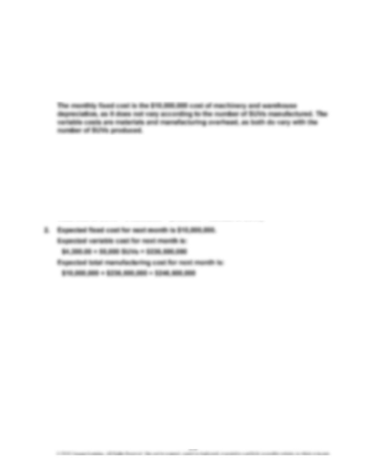
1. The cost formula takes the following form:
Total Cost = Fixed Cost + (Variable Rate × Number of SUVs)
Cost of materials per SUV is:
75,000,000 pounds/50,000 SUVs = 1,500 pounds per SUV
Given that, the material cost per SUV = $0.20 × 1,500 pounds per SUV = $300.00 per SUV.
Cost of manufacturing overhead per SUV is:
$200,000,000/50,000 SUVs = $4,000.00 per SUV
Therefore, the variable rate per SUV is $300.00 + $4,000.00 = $4,300.00.
The cost formula is:
Total Cost of SUVs = $10,000,000 + ($4,300.00 × Number of SUVs)
BRIEF EXERCISES: SET B
CHAPTER 3 Cost Behavior and Forecasting
BE 3-26
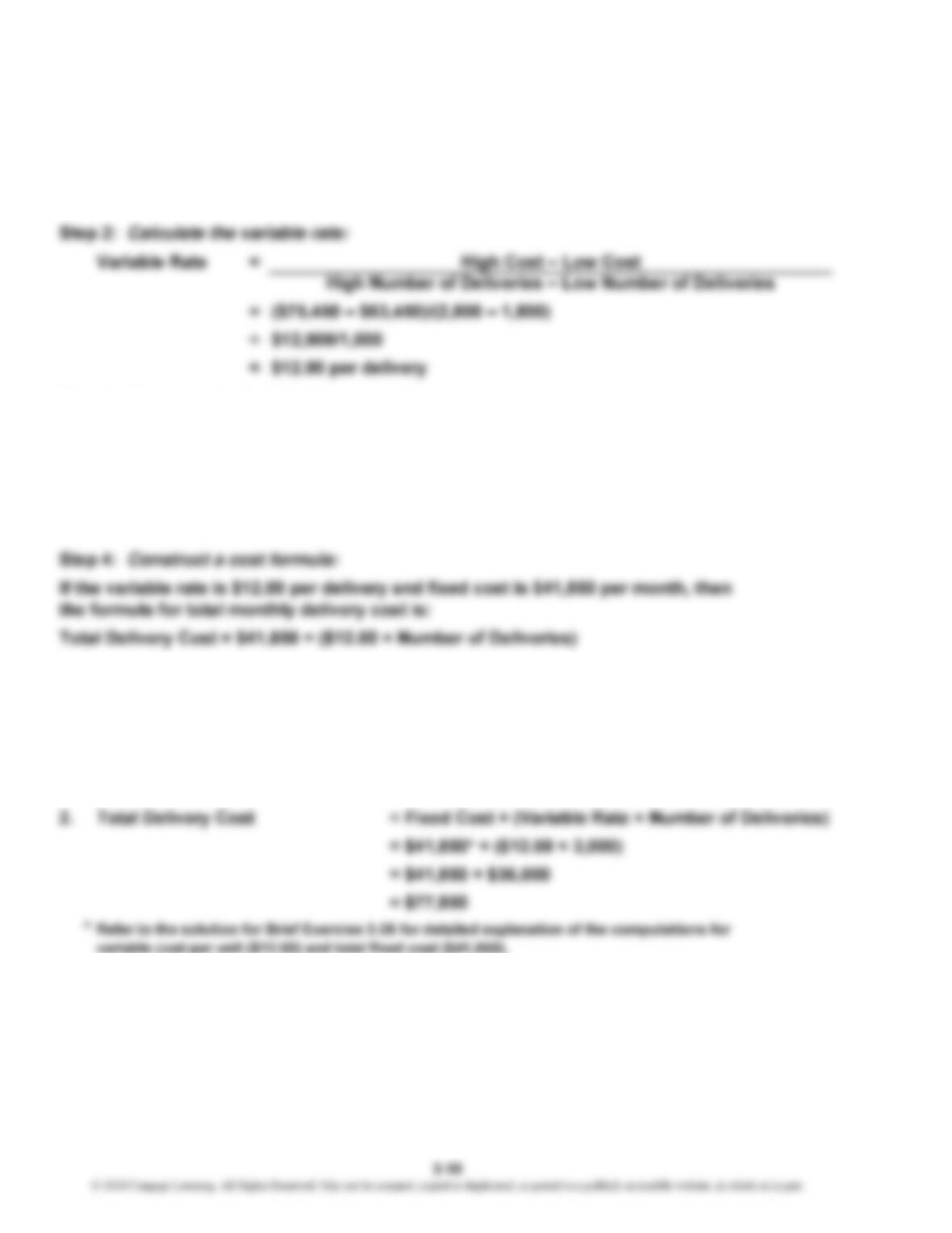
Step 1: Find the high and low points: The high number of deliveries is in November
and the low number of deliveries is in May.
Step 3: Calculate the fixed cost:
Fixed Cost = Total Cost – (Variable Rate × Number of Deliveries)
Let’s choose the low point with total cost of $63,450 and number of deliveries of 1,800.
Fixed Cost = $63,450 – ($12.00 × 1,800) = $63,450 – $21,600 = $41,850
(Hin
t
: Check your work by computing fixed cost using the high point.)
BE 3-27
1. Total Variable Delivery Cost = Variable Rate × Number of Deliveries
= $12.00* × 3,000 deliveries
= $36,000
CHAPTER 3 Cost Behavior and Forecasting
BE 3-28
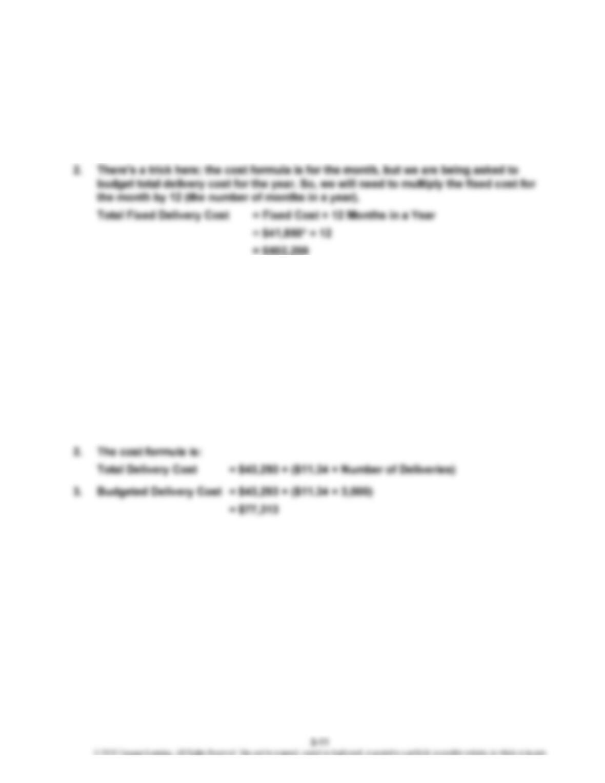
1. Total Variable Delivery Cost = Variable Rate × Number of Deliveries
= $12.00* × 3,000 deliveries
3. Total Delivery Cost = (12 × $41,850) + ($12.00 × 3,000)
= $502,200 + $36,000
*Refer to the solution for Brief Exercise 3-26 for detailed explanation of the computations for
variable cost per unit ($12.00) and total monthly fixed cost ($41,850).
BE 3-29
1. The fixed cost and the variable rate are given directly by regression.
Fixed Cost = $43,293
V
ariable Rate = $11.34
= $36,000
= $538,200
CHAPTER 3 Cost Behavior and Forecasting
BE 3-30
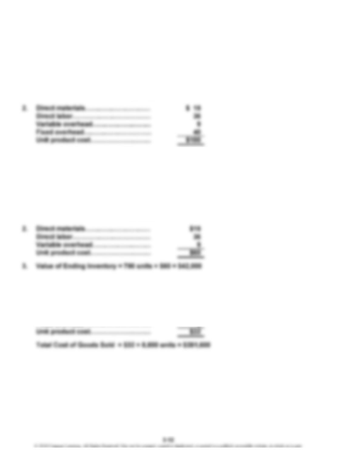
1. Units Ending Inventory = Units Beginning Inventory + Units Produced –
Units Sold
= 400 + 14,000 – 13,700
= 700 units
3.
V
alue of Ending Inventory = 700 units × $100 = $70,000
BE 3-31
1. Units Ending Inventory = Units Beginning Inventory + Units Produced –
Units Sold
= 400 + 14,000 – 13,700
= 700 units
V
V
BE 3-32
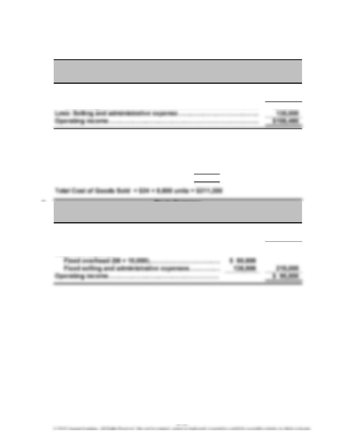
1. Direct materials………………………… $12
Direct labor……………………………… 7
V
ariable overhead……………………… 5
V
CHAPTER 3 Cost Behavior and Forecasting
BE 3-32 (Concluded)
2.
Sales ($60 × 8,800)……………………………………………………………
…
$528,000
Less: Cost of goods sold……………………………………………………
…
281,600
Gross margin…………………………………………………………..…… $246,400
BE 3-33
1. Direct materials…………………………………
…
$12
Direct labor………………………………………
…
7
V
ariable overhead………………………………
…
5
Unit product cost…………………………………
…
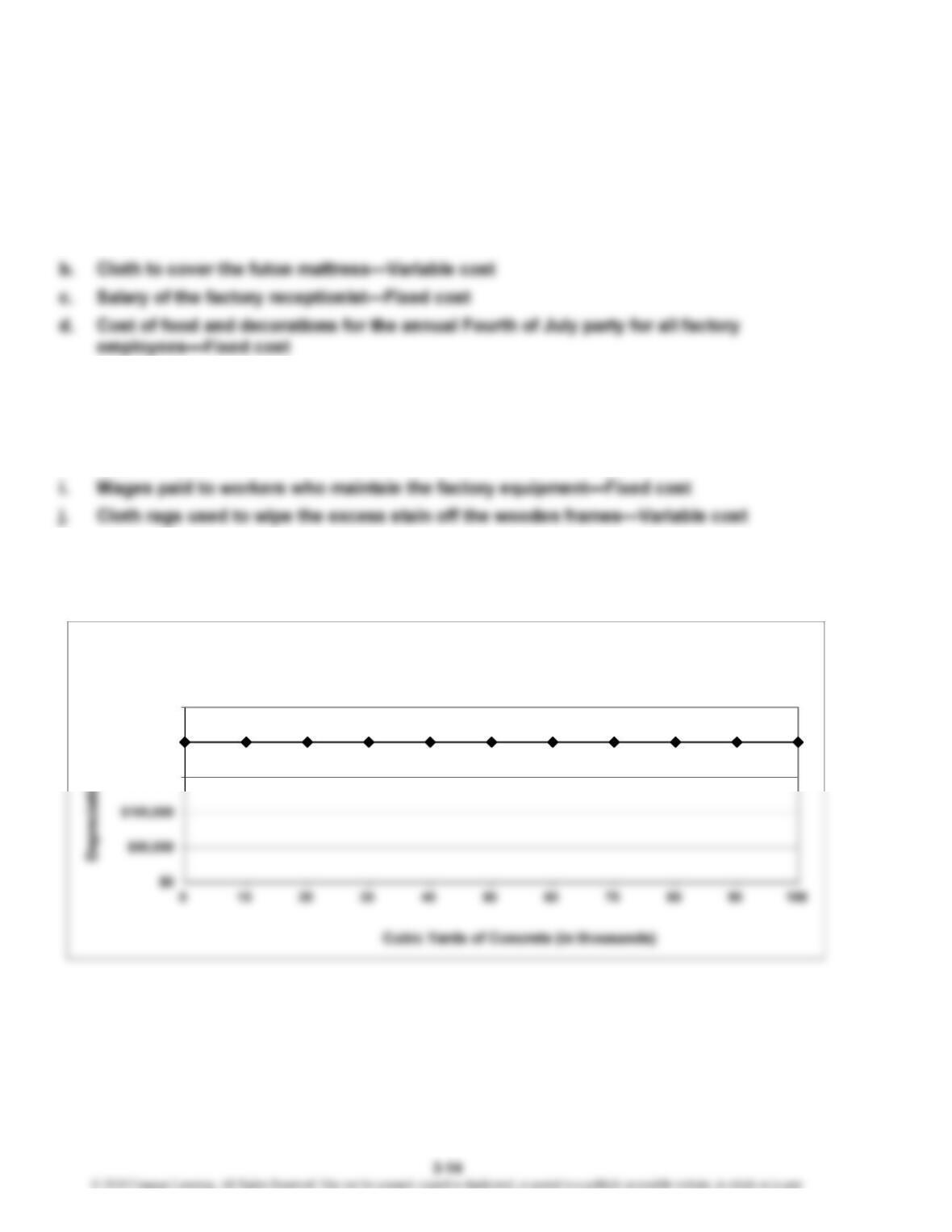
$24
2.
Sales ($60 × 8,800)………………………….…………………
…
$528,000
Less: Variable costs………………………………………….. 211,200
Contribution margin………………………………………
…
$316,800
…
Beyta Company
Income Statement under Variable Costing
For the Most Recent Year
Beyta Company
Income Statement under Absorption Costing
For the Most Recent Year
CHAPTER 3 Cost Behavior and Forecasting
E 3-34
a. Power to operate a drill (to drill holes in the wooden frames of the futons)—
V
ariable cost
e. Fuel for a forklift used to move materials in a factory—Variable cost
f. Depreciation on the factory—Fixed cost
g. Depreciation on a forklift used to move partially completed goods—Fixed cost
h. Wages paid to workers who assemble the futon frame—Variable cost
j
E 3-35
1.
EXERCISES
$150,000
$200,000
$250,000
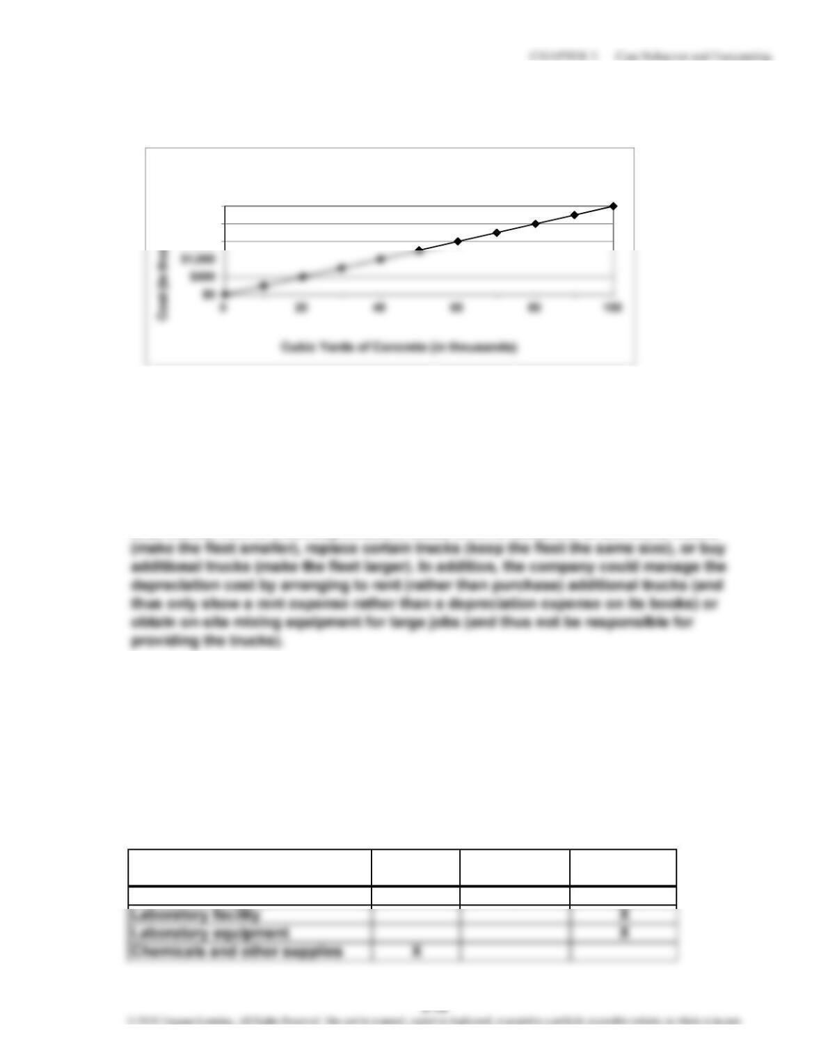
Truck Depreciation
E 3-35 (Concluded)
2.
3. Truck depreciation: Fixed cost
Raw materials cost: Variable cost
4. Truck depreciation is a fixed cost (with respect to the driver “cubic yards of cement”).
Therefore, it cannot be managed by altering the number of cubic yards of cement,
within the relevant range of course. Instead, the cost of truck depreciation could be
reduced (or increased) by changing the depreciation method that is used to allocate
the cost to each accounting period. Also, a more long-term approach to managing the
total annual cost of truck depreciation would involve decisions to sell some trucks
5. Raw materials is a variable cost (with respect to the driver “cubic yards of cement”).
Therefore, total raw materials cost likely is best reduced (or managed) either by using
fewer cubic yards of cement per job (i.e., more efficient use of cement) or by paying
less to purchase or manufacture each cubic yard of cement (i.e., more efficient
purchasing or manufacturing of cement). Also, a more long-term approach to reducing
raw materials cost would be to discover different, cheaper materials that can be used
in the business that yield the same quality of output as the existing materials.
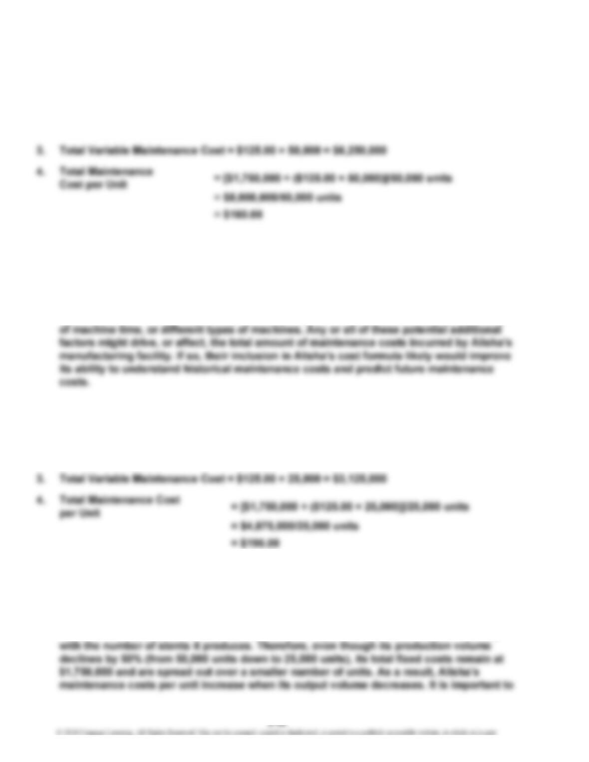
E 3-36
Technician salaries
X
Committed
Fixed Cost
Cost Category
Variable
Cost
Discretionary
Fixed Cost
$1,500
$2,000
$2,500
Raw Materials Cost
CHAPTER 3 Cost Behavior and Forecasting
E 3-37
1. Total Maintenance Cost = $1,750,000 + ($125.00 × 50,000) = $8,000,000
2. Total Fixed Maintenance Cost = $1,750,000
5. Fixed Maintenance Cost per Unit = $1,750,000/50,000 units = $35.00
6.
V
ariable Maintenance Cost per Unit = $125.00
7. Alisha management could identify (via research or conversations with its operations
personnel or employees at other similar organizations) additional drivers of maintenance
costs besides the total number of medical stents manufactured. For example, different
types of medical stents might require different types of raw materials, different amounts
E 3-38
1. Total Maintenance Cost = $1,750,000 + ($125.00 × 25,000) = $4,875,000
2. Total Fixed Maintenance Cost = $1,750,000
5. Fixed Maintenance Cost per Unit = $1,750,000/25,000 units = $70.00
6.
V
ariable Maintenance Cost per Unit = $125.00
7. The maintenance cost per unit in Exercise 3-38 is higher ($195) than in Exercise 3-37
($160) because Alisha incurs fixed costs of $1,750,000 to produce its stents. Assuming
25,000 and 50,000 stents are within the relevant range, Alisha’s fixed costs do not vary
CHAPTER 3 Cost Behavior and Forecasting
E 3-38 (Concluded)
realize that the opposite result occurs when output volume increases (i.e., total cost
per unit decreases as volume increases because fixed costs are spread out over a
greater number of units, again assuming the same relevant range). Finally, Alisha’s
E 3-39
1.
2.
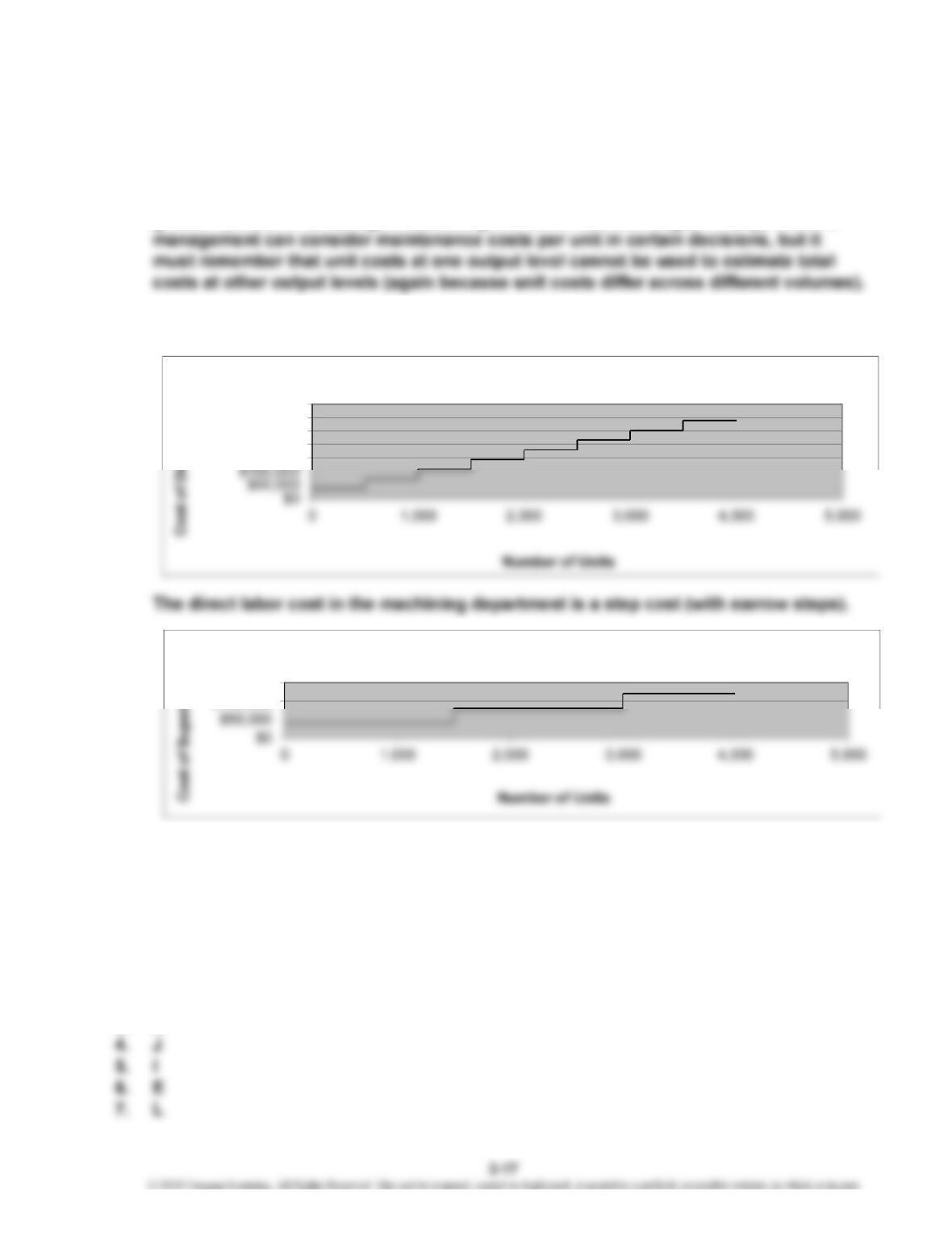
The cost of supervision for the machining department is a step cost (with wide steps).
3. Direct Labor Cost Increase = $144,000 – $108,000 = $36,000
Supervision Increase = $80,000 – $40,000 = $40,000
E 3-40
1. K
2. H
3.
A
$150,000
$200,000
$250,000
$300,000
$350,000
Direct Labor Cost
$150,000
Supervision Cost
CHAPTER 3 Cost Behavior and Forecasting
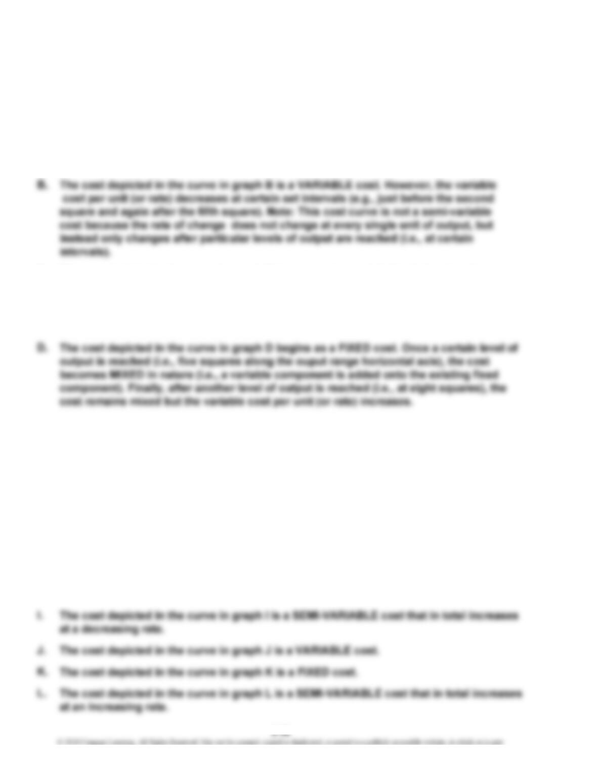
A. The cost depicted in the curve in graph A is zero up to a certain level of output (i.e., up to
three squares on the output range horizontal axis). Once a certain level of output is
reached (i.e., beyond the three squares), the cost becomes VARIABLE in nature.
However, after yet another level of output is reached (i.e., about five squares), the
variable cost per unit (or rate) decreases.
C. The cost depicted in the curve in graph C is zero up to a certain level of output (i.e., up
to three squares). Once a certain level of output is reached (i.e., at three squares), the
cost becomes a VARIABLE cost. Finally, after yet another level of output is reached (i.e.,
about five squares along the horizontal axis), the cost becomes a FIXED cost in nature
(i.e., the variable component ceases).
E. The cost depicted in the curve in graph E is a VARIABLE cost. However, the variable
cost per unit (or rate) increases at certain set intervals (e.g., just after the fourth square
and again after the seventh square). Note: This cost curve is not a semi-variable cost
because the rate of change does not change at every single unit of output, but instead
only changes after particular levels of output are reached (i.e., at certain intervals).
F. The cost depicted in the curve in graph F is a MIXED cost. However, the rate of change
(for the variable component) increases at certain set intervals (e.g., just after the fourth
square and again after the seventh square).
G. The cost depicted in the curve in graph G begins as a SEMI-VARIABLE cost that in total
increases at a decreasing rate. However, once a certain level of output is reached (i.e.,
at eight squares along the output range horizontal axis), the cost becomes a FIXED cost.
H. The cost depicted in the curve in graph H is a STEP FUNCTION cost.
E 3-41
CHAPTER 3 Cost Behavior and Forecasting
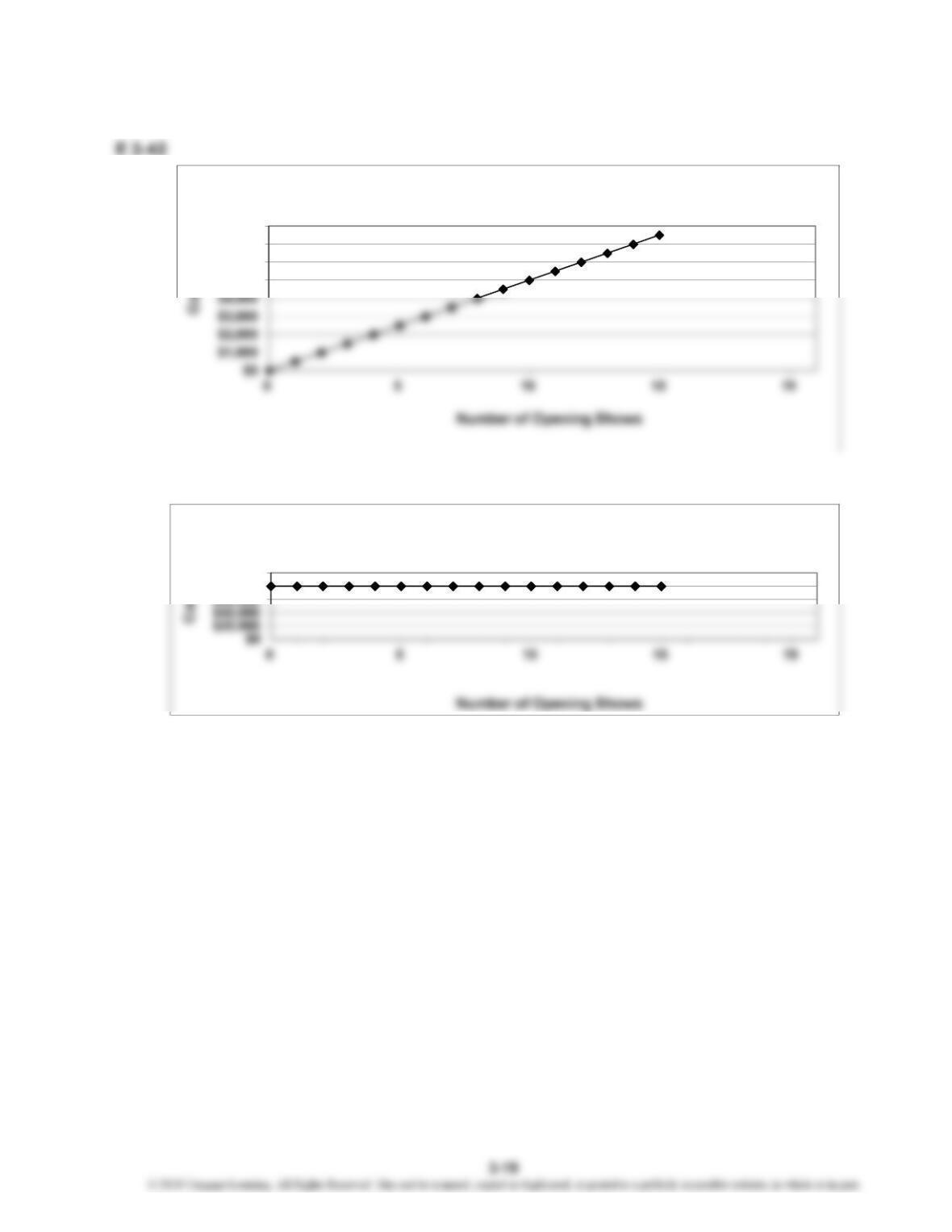
This is a strictly variable cost.
2.
This is a fixed cost.
1.
$5,000
$6,000
$7,000
$8,000
Cost of Giving Opening Shows
$80,000
$100,000
Cost of Running Gallery
CHAPTER 3 Cost Behavior and Forecasting
E 3-42 (Concluded)
3.
This is a mixed cost.
E 3-43
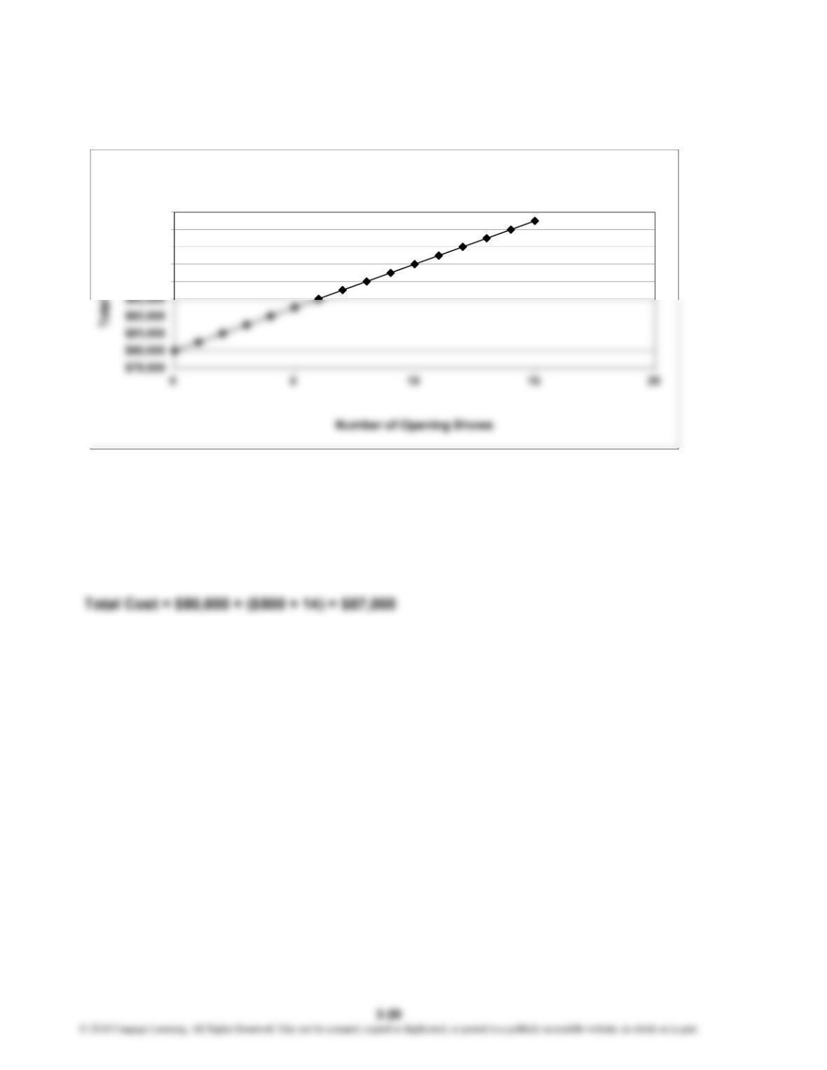
1. Total Cost = $80,000 + ($500 × Number of Opening Shows)
2. Total Cost = $80,000 + ($500 × 12) = $86,000
$84,000
$85,000
$86,000
$87,000
$88,000
Ben’s Total Costs