1. Knowledge of cost behavior allows a manager to assess changes in costs that result from
changes in activity. This allows a manager to examine the effects of choices that change activity.
For example, if excess capacity exists, bids that at least cover variable costs may be totally
appropriate. Knowing what costs are variable and what costs are fixed can help a manager make
better bids and, ultimately, better business decisions.
2. A driver is a factor that causes or leads to a change in a cost or activity; it is an output measure.
The driver for general machine maintenance cost in a factory could be machine hours. The driver
for raw materials used is the number of units produced.
3. The cost formula for monthly shipping cost is: Shipping costs 3,560
Monthly Shipping Cost = $3,560 + $6.70 × Packages Shipped Package shipped 6.70
The independent variable is packages shipped. The dependent variable is monthly shipping cost.
4. Some account categories are primarily fixed or variable. Even if the cost is mixed, either the fixed
component or the variable component is relatively small. As a result, assigning all of the cost to
either a fixed or variable category is unlikely to result in large errors. For example, depreciation on
property, plant, and equipment is largely fixed. The cost of telephone expense for the sales office,
if it consisted primarily of long-distance calls, could be seen as largely variable (variable with
respect to the number of customers).
5. Committed fixed costs are those incurred for the acquisition of long-term activity capacity and are
not subject to change in the short run. Annual resource expenditure is independent of actual
usage. For example, the cost of a factory building is a committed fixed cost. Discretionary fixed
costs are those incurred for the acquisition of short-term activity capacity, the levels of which can
be altered quickly. In the short run, resource expenditure is also independent of actual activity
usage. Salaries of engineers are an example of such an expenditure.
6. The concept of relevant range is important in dealing with step costs because if the relevant range
is contained completely within one step, the cost behaves as a fixed cost. However, if the relevant
range spans two or more steps, the accountant must be aware of the cost increase as output
goes up within the relevant range.
7. Mixed costs are usually reported in total in the accounting records. How much of the cost is fixed
and how much is variable is unknown and must be estimated.
8. The cost formula for a strictly fixed cost has only a fixed cost amount. There is no variable rate
and no independent variable. For the depreciation example, the cost formula looks like this: depreciation/year 15,000
Depreciation per Year = $15,000
9. The cost formula for a strictly variable cost has only the variable rate and independent variable.
There is no fixed component. For the electrical power example, the cost formula looks like this: electrical power cost 1.15
Electrical Power = $1.15 × Machine Hours
3
COST BEHAVIOR AND
FORECASTING
DISCUSSION QUESTIONS
CHAPTER 3 Cost Behavior and Forecasting
10. A scattergraph allows a visual portrayal of the relationship between cost and activity. It
reveals to the investigator whether a relationship may exist and, if so, whether a linear
function can be used to approximate the relationship.
11. Managers can use their knowledge of the cost relationships to estimate the fixed and
12. Because the scattergraph method is not restricted to the high and low points, it is
possible to select two points that better represent the relationship between activity and
costs, producing a better estimate of fixed and variable costs. The main advantage of the
high-low method is that it removes subjectivity from the choice process. The same line
will be produced by two different people.
13. Assuming that the scattergraph reveals that a linear cost function is suitable, then the
method of least squares selects a line that best fits the data points. The method also
provides a measure of goodness of fit so that the strength of the relationship between
cost and activity can be assessed.
14.
The best-fitting line is the one that is “closest” to the data points. This is usually
measured by the line that has the smallest sum of squared deviations from the individual
data points.
15. The only difference between absorption costing and variable costing is the way in which
16. Absorption-costing income is greater because some of the period’s fixed overhead is placed
income statement.
17. The coefficient of determination is the percentage of total variability in costs explained by
activity. As such, it is a measure of goodness of fit, the strength of the relationship
between cost and activity.
CHAPTER 3 Cost Behavior and Forecasting
3-1. c
3-2. e
3-3. b
3-4. d
3-5. a
3-6. d
3-7. c
3-8. d Total Cost = $235,000 + ($75 × 8,000) = $835,000 235,000 + 75 × 8,000 = 835,000
3-9. b
3-10. b
3-11. a
3-12. e
3-13. b
3-14. b
3-15. d
MULTIPLE-CHOICE QUESTIONS
CHAPTER 3 Cost Behavior and Forecasting
BE 3-16
1.
The cost formula takes the following form:
Total Cost = Fixed Cost + (Variable Rate × Number of Flash Drives) change here first, please →
The monthly fixed cost is the $15,000 cost of equipment depreciation, as it does not Monthly depreciation costs on P&E 15,000
vary according to the number of flash drives manufactured. The variable costs are Materials required (ounces) 10,000
materials and manufacturing overhead, as both do vary with the number of flash Material cost per ounces 3
drives produced.
Therefore, the variable rate per flash drive is $6.00 + $4.50 = $10.50 6.00 + 4.50 = 10.50
The cost formula is:
Total Cost of Flash Drives = $15,000 + ($10.50 × Number of Flash Drives) 15,000 + 10.50 × flash drives = total cost
2. Expected fixed cost for next month is $15,000. ↑ links ↓
Expected variable cost for next month is:
BRIEF EXERCISES: SET A
BE 3-17
Step 1: Find the high and low points: The high number of employee hours is in March, change here first, please → Labor Employee
and the low number of employee hours is in August. January 7,000 360
Step 2: Calculate the variable rate: February 8,140 550
Step 3: Calculate the fixed cost: August 7,531 310
Fixed Cost = Total Cost – (Variable Rate × Employee Hours) ↑ links ↓
Let’s choose the low point with total cost of $7,531 and employee hours of 310.
Fixed Cost = $7,531 – ($7.40 × 310) = $7,531 – $2,294 = $5,237 7,531 – 7.40 × 310
7,531 – 2,294 = 5,237 total fixed cost
(Hint : Check your work by computing fixed cost using the high point.)
Step 4: Construct a cost formula: ↑ links ↓
If the variable rate is $7.40 per employee hour and fixed cost is $5,237 per month, then
the formula for total monthly labor cost is:
Total Labor Cost = $5,237 + ($7.40 × Employee Hours) 5,237 + 7.40 ×
BE 3-18
1. Total Variable Labor Cost = Variable Rate × Employee Hours
= $7.40* × 675 hours 7.40 × 675 = 4,995
= $5,237* + ($7.40 × 675) 5,237 + 7.40 × 675
= $5,237 + $4,995 5,237 + 4,995 = 10,232
CHAPTER 3 Cost Behavior and Forecasting
BE 3-19
1. Total Variable Labor Cost = Variable Rate × Employee Hours
↓ link to footnote below
= $7.40* × 4,000 hours 7.40 × 4,000 = 29,600
2. There’s a trick here; the cost formula is for the month, but we are being asked to budget
labor cost for the year. So, we will need to multiply the fixed cost for the month by 12
(the number of months in a year).
Total Fixed Labor Cost = Fixed Cost × 12 Months in a Year
↓ link to footnote below
= $5,237* × 12 5,237 × 12 = 62,844
↑ links ↓
= $92,444
BE 3-20
1. The fixed cost and the variable rate are given directly by regression. intercept 4,517
Fixed Cost = $4,517 X variable 8.20
Variable Rate = $8.20 budgeted hours 675
= $10,052
= $29,600
= $62,844
CHAPTER 3 Cost Behavior and Forecasting
BE 3-21
1. Units Ending Inventory = Units Beginning Inventory + Units Produced – make changes here, please
Units Sold
=300 + 15,000 – 12,700 300 + 15,000 – 12,700 = 2,600
= 2,600 units
2.
Direct materials………………………………………………………………………………………………….
$ 20 20
Direct labor…………………………………………………………………………………………….
Variable overhead…………………………………………………………………………………………….
Fixed overhead…………………………………………………………………………………………….
BE 3-22
1. Units Ending Inventory = Units Beginning Inventory + Units Produced –
Units Sold
=300 + 15,000 – 12,700 300 + 15,000 – 12,700 = 2,600
= 2,600 units
2.
Direct materials…………………………………………………………………………………………….
$20 20
Direct labor…………………………………………………………………………………………….
Variable overhead…………………………………………………………………………………………….
BE 3-23
1.
Direct materials…………………………………………………………………………………………….
$ 9 9
Direct labor…………………………………………………………………………………………….
6 6
Variable overhead…………………………………………………………………………………………….
4 4
Fixed overhead…………………………………………………………………………………………….
5 5
CHAPTER 3 Cost Behavior and Forecasting
BE 3-23 (Concluded)
2.
Sales ($47 × 9,300)………………………………………………………………………………………………………….………………………………………..…
$437,100 47 × 9,300 = 437,100
Less: Cost of goods sold……………………………………………………………………………………………………………………………………………..
Gross margin…………………………………………………………..…………………………………………………………………………………………….
Less: Selling and administrative expense………………………….…………………………………………………………………………………………….
BE 3-24 make changes here, please
1.
Direct materials…………………………………………………………………………………………….
$ 9 9
Direct labor…………………………………………………………………………………………….
66
Variable overhead…………………………………………………………………………………………….
44
Total Cost of Goods Sold = $19 × 9,300 units = $176,700
(link)
2.
Sales ($47 × 9,300)………………………….…………………………………………………………………………………………………………………...………….
$437,100 47 × 9,300 = 437,100
Less: Variable costs…………………………………………………………………………..………………………..
176,700 176,700 ← link
Contribution margin……………………………………………………..…………………………
$260,400
Fixed overhead ($5 × 10,000) …………………………………….……………………………………………………………………………………………………………
$ 50,000 5 × 10,000 = 50,000
Fixed selling and administrative expenses…………………………………………………..………………………………………..…………….
138,000 188,000 138,000
Osterman Company
Income Statement under Variable Costing
For the Most Recent Year
(link)
Osterman Company
Income Statement under Absorption Costing
For the Most Recent Year
CHAPTER 3 Cost Behavior and Forecasting
BE 3-25
1.
The cost formula takes the following form:
Total Cost = Fixed Cost + (Variable Rate × Number of SUVs) change here first, please →
The monthly fixed cost is the $10,000,000 cost of machinery and warehouse Monthly depreciation costs on P&E 10,000,000
depreciation, as it does not vary according to the number of SUVs manufactured. The Materials required (pounds) 75,000,000
variable costs are materials and manufacturing overhead, as both do vary with the Material cost per pound .20.
number of SUVs produced.
Cost of materials per SUV is: ↓ links ↓ Manufacturing overhead resources 200,000,000
75,000,000 pounds/50,000 SUVs = 1,500 pounds per SUV 75,000,000 / 50,000 = 1,500.00 SUVs produced per month 50,000
2. Expected fixed cost for next month is $10,000,000. ↑ links ↓
Expected variable cost for next month is:
$4,300.00 × 55,000 SUVs = $236,500,000
4,300.00 × 55,000 = 236,500,000
BRIEF EXERCISES: SET B
CHAPTER 3 Cost Behavior and Forecasting
BE 3-26
Step 1: Find the high and low points: The high number of deliveries is in November change here first, please → Delivery Cost # Deliveries
and the low number of deliveries is in May. May 63,450 1,800
Step 2: Calculate the variable rate: June 67,120 2,010
Step 3: Calculate the fixed cost: December 73,300 2,725
Fixed Cost = Total Cost – (Variable Rate × Number of Deliveries) ↑ links ↓
Let’s choose the low point with total cost of $63,450 and number of deliveries of 1,800.
Fixed Cost = $63,450 – ($12.00 × 1,800) = $63,450 – $21,600 = $41,850 63,450 – 12.00 × 1,800
63,450 – 21,600 = 41,850 total fixed cost
(Hint : Check your work by computing fixed cost using the high point.)
Step 4: Construct a cost formula: ↑ links ↓
If the variable rate is $12.00 per delivery and fixed cost is $41,850 per month, then
the formula for total monthly delivery cost is:
Total Delivery Cost = $41,850 + ($12.00 × Number of Deliveries) 41,850 + 12.00 ×
BE 3-27
1. Total Variable Delivery Cost = Variable Rate × Number of Deliveries
= $12.00* × 3,000 deliveries
12.00 × 3,000 = 36,000
= $36,000 ↑ links ↓
= $41,850* + ($12.00 × 3,000) 41,850 + 12.00 × 3,000
= $41,850 + $36,000 41,850 + 36,000 = 77,850
CHAPTER 3 Cost Behavior and Forecasting
BE 3-28
1. Total Variable Delivery Cost = Variable Rate × Number of Deliveries
↓ link to footnote below
= $12.00* × 3,000 deliveries 12.00 × 3,000 = 36,000
2. There’s a trick here; the cost formula is for the month, but we are being asked to
budget total delivery cost for the year. So, we will need to multiply the fixed cost for
the month by 12 (the number of months in a year).
Total Fixed Delivery Cost = Fixed Cost × 12 Months in a Year
↓ link to footnote below
= $41,850* × 12 41,850 × 12 = 502,200
↑ links ↓
= $538,200
BE 3-29
1. The fixed cost and the variable rate are given directly by regression. intercept 43,293
Fixed Cost = $43,293 X variable 11.34
Variable Rate = $11.34 budgeted # of deliveries 3,000
2. The cost formula is: ↓ links ↓ 77,313
Total Delivery Cost = $43,293 + ($11.34 × Number of Deliveries) 43,293 + 11.34 × # of deliveries = ?
= $77,313
= $36,000
= $502,200
BE 3-30
1. Units Ending Inventory = Units Beginning Inventory + Units Produced – make changes here, please
Units Sold
=400 + 14,000 – 13,700 400 + 14,000 – 13,700 = 700
= 700 units
Direct materials………………………………………………………………………………………………….
Direct labor…………………………………………………………………………………………….
Variable overhead…………………………………………………………………………………………….
Fixed overhead…………………………………………………………………………………………….
Unit product cost…………………………………………………………………………………………….
BE 3-31
1. Units Ending Inventory = Units Beginning Inventory + Units Produced –
Units Sold
=400 + 14,000 – 13,700 400 + 14,000 – 13,700 = 700
= 700 units
2.
Direct materials…………………………………………………………………………………………….
$15 15
Direct labor…………………………………………………………………………………………….
36 36
Variable overhead…………………………………………………………………………………………….
9 9
Unit product cost…………………………………………………………………………………………….
$60
BE 3-32
1.
Direct materials…………………………………………………………………………………………….
$12 12
Direct labor…………………………………………………………………………………………….
7 7
Variable overhead…………………………………………………………………………………………….
5 5
Fixed overhead…………………………………………………………………………………………….
Unit product cost…………………………………………………………………………………………….
$32
BE 3-32 (Concluded)
2.
Sales ($60 × 8,800)………………………………………………………………………………………………………….………………………………………..…
$528,000 60 × 8,800 = 528,000
Less: Cost of goods sold……………………………………………………………………………………………………………………………………………..
← link
Less: Selling and administrative expense………………………….…………………………………………………………………………………………….
Operating income…………………………………………………………………………………………………………………………………………….…………
BE 3-33 make changes here, please
1.
Direct materials…………………………………………………………………………………………….
$12 12
Direct labor…………………………………………………………………………………………….
7 7
Variable overhead…………………………………………………………………………………………….
5 5
Unit product cost…………………………………………………………………………………………….
$24
Total Cost of Goods Sold = $24 × 8,800 units = $211,200 24 × 8,800 = 211,200
2.
Sales ($60 × 8,800)………………………….……………………………………………………………………………………………………………………………….
$528,000 60 × 8,800 = 528,000
Less: Variable costs…………………………………………………………………………..………………………..
211,200 211,200
← link
Operating income…………………………………………………………………………..………………………….
Beyta Company
Income Statement under Variable Costing
For the Most Recent Year
(link)
Beyta Company
Income Statement under Absorption Costing
For the Most Recent Year
(link)
CHAPTER 3 Cost Behavior and Forecasting
E 3-34
a. Power to operate a drill (to drill holes in the wooden frames of the futons)—
Variable cost
e. Fuel for a forklift used to move materials in a factory—Variable cost
f. Depreciation on the factory—Fixed cost
g. Depreciation on a forklift used to move partially completed goods—Fixed cost
h. Wages paid to workers who assemble the futon frame—Variable cost
change here, please
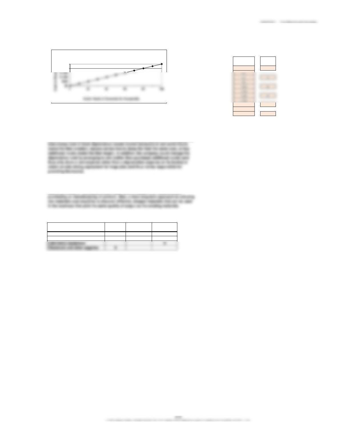
E 3-35 depreciation concrete
1. cost (cubic yards)
200,000 0
200,000 10
200,000 20
200,000 30
200,000 40
200,000 50
200,000 60
EXERCISES
$150,000
$200,000
$250,000
Truck Depreciation
E 3-35 (Concluded)
2. change here first, please →
raw materials cubic yds
cost concrete
0 0
2,000 80
3. Truck depreciation: Fixed cost 2,250
Raw materials cost: Variable cost 2,500 100
4. Truck depreciation is a fixed cost (with respect to the driver “cubic yards of cement”).
Therefore, it cannot be managed by altering the number of cubic yards of cement,
within the relevant range of course. Instead, the cost of truck depreciation could be
reduced (or increased) by changing the depreciation method that is used to allocate
5. Raw materials is a variable cost (with respect to the driver “cubic yards of cement”).
Therefore, total raw materials cost likely is best reduced (or managed) either by using
fewer cubic yards of cement per job (i.e., more efficient use of cement) or by paying
E 3-36
Technician salaries
Laboratory facility
X
X
Committed
Fixed Cost
X
Cost Category
Variable
Cost
Discretionary
Fixed Cost
$2,000
$2,500
Raw Materials Cost
CHAPTER 3 Cost Behavior and Forecasting
change here first, please
E 3-37
1. Total Maintenance Cost = $1,750,000 + ($125.00 × 50,000) = $8,000,000 1,750,000 + 125.00 × 50,000 = 8,000,000 maint. fixed cost 1,750,000
2.
Total Fixed Maintenance Cost = $1,750,000
1,750,000 ← links ↓ maint. variable cost 125.00
3. Total Variable Maintenance Cost = $125.00 × 50,000 = $6,250,000 125.00 × 50,000 = 6,250,000 stents 50,000
4. Total Maintenance 1,750,000 + 125.00 × 50,000 /50,000
Cost per Unit
= $8,000,000/50,000 units
8,000,000 /50,000 = 160.00
= [$1,750,000 + ($125.00 × 50,000)]/50,000 units
5. Fixed Maintenance Cost per Unit = $1,750,000/50,000 units = $35.00 1,750,000 /50,000 = 35.00
6. Variable Maintenance Cost per Unit = $125.00 125.00 ← link
7. Alisha management could identify (via research or conversations with its operations
personnel or employees at other similar organizations) additional drivers of maintenance
costs besides the total number of medical stents manufactured. For example, different
types of medical stents might require different types of raw materials, different amounts
of machine time, or different types of machines. Any or all of these potential additional
its ability to understand historical maintenance costs and predict future maintenance
E 3-38
1. Total Maintenance Cost = $1,750,000 + ($125.00 × 25,000) = $4,875,000 1,750,000 + 125.00 × 25,000 = 4,875,000 maint. fixed cost 1,750,000
2.
Total Fixed Maintenance Cost = $1,750,000
maint. variable cost 125.00
3. Total Variable Maintenance Cost = $125.00 × 25,000 = $3,125,000 125.00 × 25,000 = 3,125,000 stents 25,000
4. Total Maintenance Cost 1,750,000 + 125.00 × 25,000 /25,000
per Unit
= $4,875,000/25,000 units
4,875,000 /25,000 = 195.00
= $195.00 ↑ links ↓
5. Fixed Maintenance Cost per Unit = $1,750,000/25,000 units = $70.00 1,750,000 /25,000 = 70.00
6. Variable Maintenance Cost per Unit = $125.00 125.00 ← link
7. The maintenance cost per unit in Exercise 3-38 is higher ($195) than in Exercise 3-37
($160) because Alisha incurs fixed costs of $1,750,000 to produce its stents. Assuming
with the number of stents it produces. Therefore, even though its production volume
declines by 50% (from 50,000 units down to 25,000 units), its total fixed costs remain at
maintenance costs per unit increase when its output volume decreases. It is important to
= [$1,750,000 + ($125.00 × 25,000)]/25,000 units
CHAPTER 3 Cost Behavior and Forecasting
E 3-38 (Concluded)
realize that the opposite result occurs when output volume increases (i.e., total cost
per unit decreases as volume increases because fixed costs are spread out over a
greater number of units, again assuming the same relevant range). Finally, Alisha’s
management can consider maintenance costs per unit in certain decisions, but it
must remember that unit costs at one output level cannot be used to estimate total
costs at other output levels (again because unit costs differ across different volumes).
E 3-39
1.
change here first, please → units units machining machining
produced produced direct labor cost duration_DL height_DL supervision cost duration_S height_S
0–500 0 36,000 501 0 40,000 501 0
The direct labor cost in the machining department is a step cost (with narrow steps).
2.
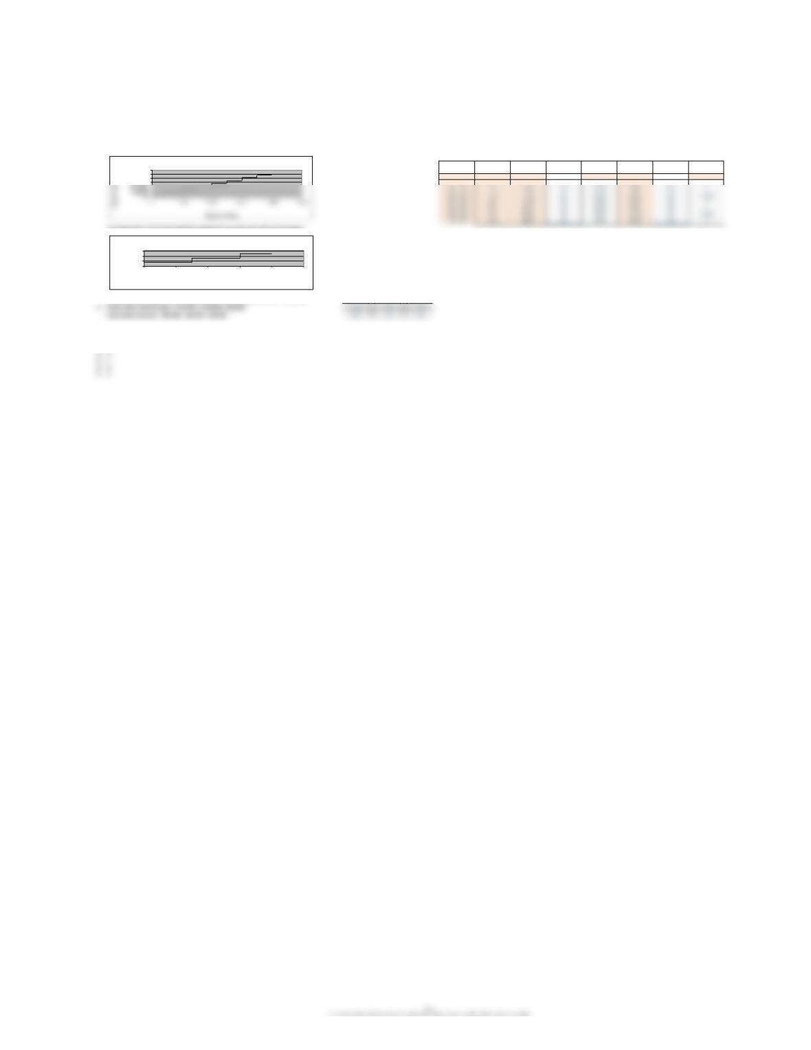
The cost of supervision for the machining department is a step cost (with wide steps).
Supervision Increase = $80,000 – $40,000 = $40,000 80,000 – 40,000 = 40,000
E 3-40
1. K
2. H
3. A
4. J
5. I
6. E
7. L
$250,000
$300,000
$350,000
Direct Labor Cost
$0
$50,000
$100,000
$150,000
0 1,000 2,000 3,000 4,000 5,000
Cost of Supervision
Number of Units
Supervision Cost

CHAPTER 3 Cost Behav ior and Forecas ting
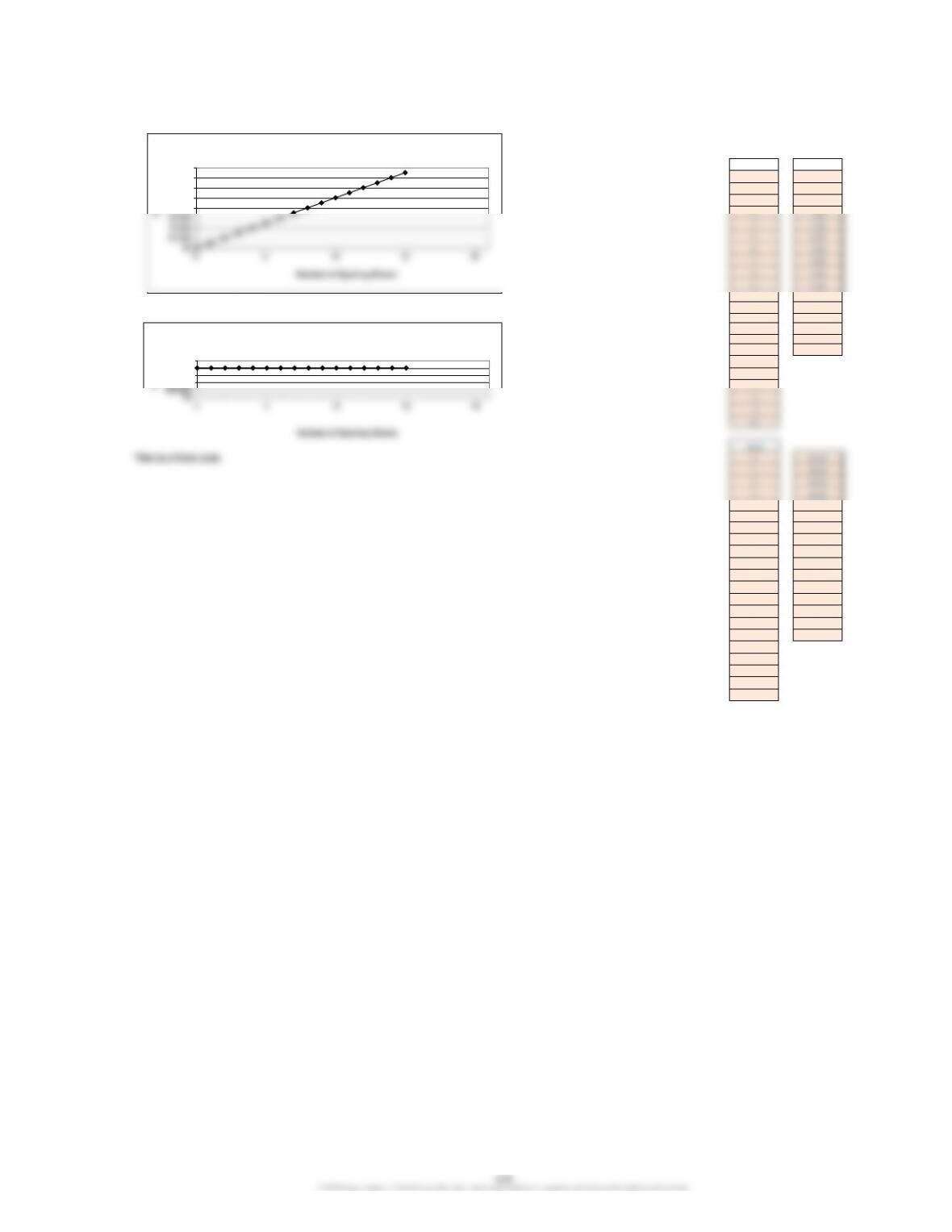
reache d( ie beyond the th ree square s) the cost beco mes VARIABLEin nature
Howeve r after yet an other leve l of output is re ached (i e about five square s) the
variable cost p er unit (or r ate) decre ases
B. The cos t depicted in the curve in graph B is a VARIABLEcos t However the variable
cost pe r unit (or rate ) decreas es at cert ains et inter vals (e g jus t before t he second
square an dagain afte r the fifth square) Note: This cost curve is not a sem i variable
cost be cause the r ate of change doe s not change at eve ry single unit o f output but
inste ad only changes afte r particular leve ls of output are reached (i e at certain
inter vals)
C. The cos t depicted in the curve in graph C is zero up to a ce rtain level of out put (i e up
to thre e square s) Once a certain le vel of output is reached (i e at thre e square s) the
cost be comes a VARIABLEcos t Finally afte r yet anothe r level of outp ut is reached ( ie
about five squar es along the horizont alaxis) th e cost become s aFIXEDcost in natur e
(i e the variable com ponent ceas es)
D. The cos t depicted in the curve in graph D beg ins as a FIXEDcos t Once a certain leve l of
output is re ached (ie five sq uares along the ouput range h orizontal axis) the cost
becom es MIXEDin nat ure (i e a var iable compone nt is added ont o the existin g fixed
compon ent) Finally after anothe r level of out put is reache d (i e at eight s quares) t he
cost re mains m ixed but the variable cost per u nit (or rate) incr eases
E.
The cos t depicted in the curve in graph E is a VARIABLEcos t How ever th e variable
cost pe r unit (or rate ) increase s at certain se t intervals ( e g just afte r the four th square
and again after the se venth square ) Note: This cost curve is not a se mi variable cost
because the rate of change does not change at eve ry single unit o f output but inst ead
only changes af ter particular le vels of outpu t are reache d (i e at cert ainin tervals)
F. The cost de picted in the curve in graph Fis a MIXEDcos t How ever the rate o fchang e
(for the variable comp onent) incre ases at cer tain set inte rvals (e g jus t after the fourth
square and again after th e seven th square )
increas es at a decre asing rate How ever once a certain leve lo f output is re ached (i e
at eight squar es along the output range hor izontal axis) the cost becom es a FIXEDcos t
H. The cos t depicted in the curve in graph H is a STEP FUNCTIONcost
K. The cos t depicted in the curve in graph K is a FIXEDcost
at an increas ing rate
CHAPTER 3 Cost Behavior and Forecasting
E 3-42
change here, please
shows cost
0 0
1500
2 1,000
10 5,000
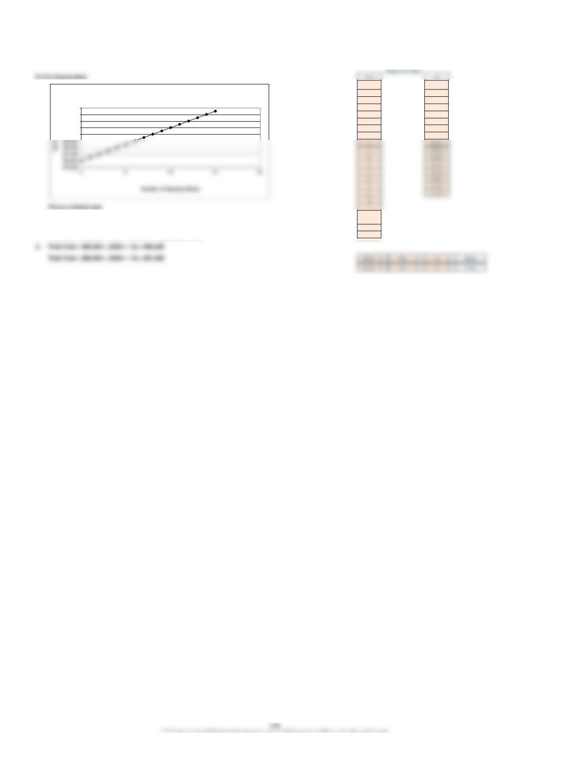
This is a strictly variable cost. 11 5,500
12 6,000
2. 13 6,500
14 7,000
15 7,500
15
16
4 80,000
5 80,000
6 80,000
7 80,000
8 80,000
9 80,000
10 80,000
11 80,000
12 80,000
13 80,000
14 80,000
15 80,000
16
17
18
19
20
1.
$4,000
$5,000
$6,000
$7,000
$8,000
Cost of Giving Opening Shows
$60,000
$80,000
$100,000
Cost of Running Gallery
CHAPTER 3 Cost Behavior and Forecasting
3. 0 80,000
1 80,500
2 81,000
3 81,500
4 82,000
5 82,500
6 83,000
18
E 3-43 19
1. Total Cost = $80,000 + ($500 × Number of Opening Shows) 20
$84,000
$85,000
$86,000
$87,000
$88,000
Ben’s Total Costs