
CHAPTER 3 Cost Behavior and Forecasting
E 3-44
1. The high point is March with 3,500 appointments. The low point is May March 3,500 ← links
Fixed Cost = $1,790 – ($0.50 × 1,500) = $1,040 1,790 – 0.50 × 1,500 = 1,040 August 3,000 2,640
3. Total Tanning Service Cost = $1,040 + ($0.50 × Number of Appointments) ↑ links ↓ ↓ links ↓ September 2,500
4. Total Predicted Cost for September = $1,040 + ($0.50 × 2,500) = $2,290 1,040 + 0.50 × 2,500 = 2,290
Total Fixed Cost for September = $1,040 ↑ links ↓
Total Predicted Variable Cost for September = $0.50 × 2,500 = $1,250 0.50 × 2,500 = 1,250
5. Using the high-low method means that Luisa’s estimate of the cost formula (and
therefore the cost behavior patterns) is based on only two data points and ignores
all of the other data. She should investigate to be sure that neither the high nor the
change here, please
CHAPTER 3 Cost Behavior and Forecasting
change here, please
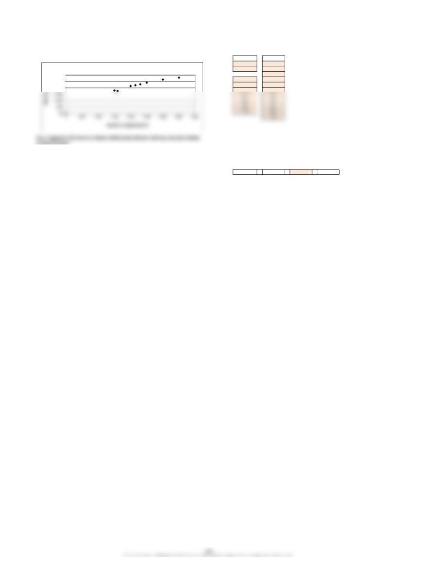
E 3-45 cost appointmts
0 0
1,754 1,600
1,000
1,790 1,500
2,140 2,000
of appointments.
E 3-46
1. Total Cost of Tanning Services = $1,016 + ($0.53 × Number of Appointments) ↓ links ↓
2. Total Predicted Cost for September = $1,016 + ($0.53 × 2,500) = $2,341 1,016 + 0.53 × 2,500 = 2,341
$2,000
$2,500
$3,000
Scattergraph of Tanning Services
CHAPTER 3 Cost Behavior and Forecasting
E 3-47
1. Airplane depreciation:
change here plea se (some are links)
Variable Rate = ($18,000,000 – $18,000,000)/(44,000 – 28,000) = $0
18,000,000 – 18,000,000 / 44,000 – 28,000 = 0
Fixed Cost = $18,000,000 – ($0 × 44,000) = $18,000,000
18,000,000 – 0 × 44,000 = 18,000,00 0
2. Total Cost of Airplane Depreciation = $18,000,000 18,000,000
Variable Rate = ($445,896,000 – $283,752,000)/(44,000 – 28,000) = $10,134
Fixed Cost = $445,896,000 – ($10,134 × 44,000) = $0
5. Airplane maintenance:
Variable Rate = ($15,792,000 – $11,504,000)/(44,000 – 28,000) = $268
15,792,000 – 11,504,000 / 44,000 – 28,000 = 268
Fixed Cost = $15,792,000 – ($268 × 44,000) = $4,000,000
15,792,000 – 268 × 44,000 = 4,000,000
6. Total cost of airplane maintenance:
$4,000,000 + ($268 × Number of Airplane Flight Hours)
4,000,000 + 268 × ? =
CHAPTER 3 Cost Behavior and Forecasting
change here first, please
E 3-48 ↓ links ↓
1. Total Annual Cost of Airplane Depreciation = 12 × $18,000,000 12 × 18,000,000 = 216,000,000 depreciation 18,000,000
= $216,000,000 ↓ links ↓ cost of fuel 10,134
Total Annual Cost of Fuel = $10,134 × (Annual Number of Airplane Flight Hours) 10,134 × ? = months 12
Total Annual Cost of Airplane Maintenance = ↓ links ↓ variable maint. rate 268
(12 × $4,000,000) + ($268 × Number of Airplane Flight Hours) 12 × 4,000,000 + 268 fixed maint. rate 4,000,000
Note: Fixed and variable costs, based on monthly data, are computed in × flight hours flight hours 480,000
Exercise 3-47. ↓ links ↓
E 3-49 ↓ links ↓
1. Total Cost of Receiving = $147,400 + ($210 × Number of Parts Inspected) 147,400 + 210 ×
2. Independent variable—number of parts inspected change here first, please → slope 210
Dependent variable—total cost of receiving parts inspected 6,800
total cost of fuel
number of parts inspected
E 3-50
1. Total Annual Cost of Receiving: change here please (some are links)
= (12 × $147,400) + ($210 × Number of Parts Inspected in a Year)
12 × 147,400 + 210 ×
= $1,768,800 + ($210 × Number of Parts Inspected in a Year)
2. Total Annual Cost of Receiving = $1,768,800 + ($210 × 70,000) 1,768,800 + 210 × 70,000 =
E 3-51 change here first, please →
1.
Overhead cost……………………………………………………………….
Dependent variable Fixed cost 150,000 quarters 3
$150,000………………………………………………………………………………………………
Fixed cost (intercept) Variable cost 52 months 12
$52………………………………………………………………………………………………
Variable rate (slope) labor hours 8,000 23,000
Direct labor hours………………………………………………………………………………………………………………….
Independent variable ↓ links ↓ machine hours 99,000
2. Next Month’s Budgeted Overhead Cost = $150,000 + ($52 × 8,000) 150,000 + 52 × 8,000 =
3.
Next Quarter’s Budgeted Overhead Cost
4. Next Year’s Budgeted Overhead Cost = (12 × $150,000) + ($52 × 99,000) 12 × 150,000 + 52 × 99,000
no. of parts inspected
566,000

CHAPTER 3 Cost Behavior and Forecasting
(links)
E 3-52 make changes here, please
1. Unit Direct Materials Cost = $80,000/20,000 units = $4.00 80,000 / 20,000 = 4.00 Direct materials 80,000
Unit Direct Labor Cost = $101,400/20,000 units = $5.07 101,400 / 20,000 = 5.07 Direct labor 101,400
Unit Variable Overhead Cost = $15,600/20,000 units = $0.78 15,600 / 20,000 = 0.78 Variable overhead 15,600
Unit direct materials cost………………………………………………………………………………………………………………………………
Unit direct labor cost………………………………………………………………………………………………………………………
Unit variable overhead cost………………………………………………………………………………………………………………………
Unit fixed overhead cost………………………………………………………………………………………………………………………
3. Ending Inventory in Units = 20,000 – 18,900 = 1,100 units 20,000 – 18,900 = 1,100
4. Absorption-Costing Ending Inventory = $12.58 × 1,100 units = $13,838 12.58 × 1,100 = 13,838
E 3-53 (links) make changes here, please
1.
Unit direct materials cost ($123,000/50,000 units)………………………………………………………………………………………………………………………
$2.46 123,000 / 50,000 = 2.46 Units produced 50,000
Unit direct labor cost ($93,000/50,000 units)………………………………………………………………………………………………………………………
Unit variable overhead cost ($65,000/50,000 units)………………………………………………………………………………………………………………………
CHAPTER 3 Cost Behavior and Forecasting
E 3-54
← links make changes here, please
1.
Unit direct materials cost………………………………………………………………………………………………………………………
$ 9.95 Unit direct materials 9.95
Unit direct labor cost………………………………………………………………………………………………………………………
2.75 Unit direct labor 2.75
Unit variable overhead cost………………………………………………………………………………………………………………………
1.65 Unit variable overhead 1.65
Unit fixed overhead cost………………………………………………………………………………………………………………………
2.50 Unit fixed overhead* 2.50
Absorption cost per unit………………………………………………………………………………………………………………………
$16.85 Unit selling expense (variable) 2.00
Unit direct materials cost………………………………………………………………………………………………………………………
Unit direct labor cost………………………………………………………………………………………………………………………
Unit variable overhead cost………………………………………………………………………………………………………………………
Variable cost per unit………………………………………………………………………………………………………………………
$14.35 SP 32
3. Absorption-costing income: Units produced 30,000
Sales ($32 × 28,700)…………………………………………………………………………………………………………………………………………………………
$918,400 32 × 28,700 = 918,400
Less: Cost of goods sold ($16.85 × 28,700)…………………………………………………………………………………………………………………………….
483,595 16.85 × 28,700 = 483,595
Gross margin……………………………………..………………………………………………………………………………………………………………
$434,805
Less:
Variable selling expense ($2 × 28,700)……………………………………………………………………………………………………………………………….
$ 57,400 2 × 28,700 = 57,400
Fixed selling expense……………………………………………………………………………………………………………………………………………………
65,500
Fixed administrative expense………………….………………………………………………………………………………………………………………………
231,000 353,900
Operating income……………………………………………………………………………………………………………………………………………………………
$ 80,905
4. Variable-costing income:
Sales ($32 × 28,700)…………………………………………………………………………………………………………………………………………………………
$918,400 32 × 28,700 = 918,400
Cost of goods sold ($14.35 × 28,700)…………………………………………………………………………………………………………………………….
Selling expense ($2.00 × 28,700)……..………………………………………………………………………………………………………………………………….
Contribution margin……………………………….………………………………………………………………………………………………………………………
Fixed overhead ($2.50 × 30,000)……………………………………………………………………………………………………………………………………….
Selling and administrative expenses………..………………………………………………………………………………………………………………………
Operating income…………………………………..…………………………………………………………………………………………………………………
$ 77,655

CHAPTER 3 Cost Behavior and Forecasting
E 3-55
1. SUMMARY OUTPUT
change here first, please →DL hours O/H cost
January 689 5,550
Multiple R 0.95657699 February 700 5,590
R Square 0.915039537 March 720 5,650
df SS MS F Significance F August 675 5,608
Regression 1 50588.87585 50588.87585 64.62108425 0.000198083
Residual 6 4697.124145 782.8540242 Direct labor hours for September 700
Total 7 55286
Coefficients Standard Error t Stat P-value Lower 95% Upper 95% Lower 95.0% Upper 95.0%
Intercept 4315.593336 158.0347739 27.30787174 1.59382E-07 3928.896176 4702.290497 3928.896176 4702.290497
DL hours 1.846241957 0.229668533 8.038724044 0.000198083 1.284263303 2.40822061 1.284263303 2.40822061
2. Overhead Cost = $4,316 + ($1.85 × Number of Direct Labor Hours)
3. The R² is 0.915, or 91.5%. In other words, 91.5% of the variation in the overhead costs from month to month
can be explained by the variability in the number of direct labor hours. Another factor (or factors) accounts
Regression Statistics

CHAPTER 3 Cost Behavior and Forecasting
CHAPTER 3 Cost Behavior and Forecasting
E 3-56
1. SUMMARY OUTPUT
change here first, please →
Multiple R 0.917226463 January 100 1,200
R Square 0.841304384 February 550 1,800
Adjusted R Square 0.825434822 March 85 1,100
Standard Error 164.5461114 April 115 1,050
Observations 12 May 160 1,190
Coefficients Standard Error t Stat P-value Lower 95% Upper 95% Lower 95.0% Upper 95.0% November 260 1,400
Intercept 942.1029802 88.16653478 10.68549402 8.62887E-07 745.6556994 1138.550261 745.6556994 1138.550261 December 450 2,200
Deliveries 1.78781384 0.245543354 7.28105163 2.6597E-05 1.240709154 2.334918525 1.240709154 2.334918525
2. Delivery Cost = $942 + ($1.79 × Number of Deliveries) 300
3. The R² is 0.841, or 84.1%. In other words, 84.1% of the variation in the monthly cost of delivery from month to month
can be explained by the variability in the number of deliveries. Another factor (or factors) accounts for just under 16%
of the variability in monthly delivery cost. This means that the number of deliveries is a fairly good predictor of the
cost.
Regression Statistics
deliveries
CHAPTER 3 Cost Behavior and Forecasting
P 3-57
1. a. Mixed cost
b. Variable cost
c. Variable cost
d. Step cost with narrow steps
2. a. While the contract stays the same ($150 per month plus $15 per hour of technical
time), the company’s need for computer technical help is so stable that the same
number of hours are required each month. Now, the cost is essentially fixed.
b. The company drives the vehicles on identical trips each month. Thus, the mileage
and type of trip (highway versus in town) never vary. Now, the cost is essentially
fixed.
e. Suppose that the dental office is located in a large shopping mall that charges rent
based on the level of sales. Rent would be variable.
f. If the law office expanded and an additional, temporary receptionist was hired on
days with a heavy volume of appointments, the cost would be mixed.
g. If the individuals working behind the counter are assured that their complete shift
would be worked once they arrive, the cost would be a step cost (assumes more
counter help could be called in if demand rose).
h. If the hygienists were paid based on number of patients seen, the cost would be
PROBLEMS

CHAPTER 3 Cost Behavior and Forecasting
P 3-58
a. This must be the high-low method because she has only two data points (one for
each year).
b. This is the method of least squares done on a personal computer. While it is
possible to use a personal computer to do the other methods, it is unlikely that
Francis would have gone to all the trouble of entering 60 months of data simply
P 3-59
a. Variable cost
b. Committed fixed cost
c. Discretionary fixed cost
d. Discretionary fixed cost
e. Discretionary fixed cost
CHAPTER 3 Cost Behavior and Forecasting
change here, please
P 3-60 orders
1. 0
700 15,000
900 16,000
1,000 18,000
1,100 21,000
1,200 17,000
1,300 25,000
1,400 24,000
2. Using the high-low method: ↓ links ↓ ↓ links ↓
Variable Receiving Cost = ($27,000 – $15,000)/(1,700 – 700) = $12 27,000 – 15,000 / 1,700 – 700 = 12
Fixed Receiving Cost = $15,000 – ($12 × 700) = $6,600 15,000 – 12 × 700 = 6,600
Predicted cost for 1,450 receiving orders: ↓ links ↓
Receiving Cost = $6,600 + ($12 × 1,450) = $24,000 6,600 + 12 × 1,450 = 24,000
Receiving Cost for the Year = (12 × $6,600) + ($12 × 18,000) 12 × 6,600 + 12 × 18,000 = 295,200
$20,000
$25,000
$30,000
$35,000
Scattergraph of Receiving Activity
CHAPTER 3 Cost Behavior and Forecasting
P 3-61 ↓ links ↓
change here first, please →
1. Receiving Cost = $3,212 + ($15.15 × Number of Receiving Orders) 3,212 + 15.15 × orders intercept 3,212
2.
Receiving Cost = $3,212 + ($15.15 × 1,450) = $25,180
3,212 + 15.15 × 1,450 = 25,180 slope 15.15
= $9,636 + $70,448*
P 3-62
1. Salaries:
Senior accountant—fixed
Office assistant—fixed
Internet and software subscriptions—mixed
Consulting by senior partner—variable
Depreciation (equipment)—fixed
Rent (offices)—fixed

CHAPTER 3 Cost Behavior and Forecasting
P 3-62 (Concluded)
2. Internet and software subscriptions: ↓ links ↓ ↓ links ↓
change here first, please →
Variable Rate = ($850 – $700)/(150 – 120) = $5
850 – 700 /150 – 120 = 5.00 5
Fixed Amount = $850 – ($5 × 150) = $100
850 – 5.00 × 150 = 100 100
Variable Rate = ($1,100 – $905)/(150 – 120) = $6.50
Fixed Amount = $1,100 – ($6.50 × 150) = $125
Fixed Amount = $365 – ($1.10 × 150) = $200
Unit Variable consulting 1,200 1,500
Fixed Cost depreciation (equip) 2,400 2,400
3. Salaries: supplies 905 1,100
Senior accountant……………………………………………………………………………………………………………………………………….
$2,500 — admin 500 500
Office assistant…………………………………………………………………………………………………………………………………………..
1,200 — rent (offices) 2,000 2,000
Internet and software subscriptions………………………………………………………………………………………….
100 $ 5.00 utilities 332 365
Consulting by senior partner…………………………………………………………………………………………………..
— 10.00 prof. hrs. per month 140
Depreciation (equipment)………………………………………………………………………………………………………
2,400 — prof. hrs. per month 170
Rent (offices)………………………………………………………………………………………………………………………
Total Clinic Cost = $9,025 + ($22.60 × Professional Hours)
For 140 professional hours: ↓ links ↓
Clinic Cost = $9,025 + ($22.60 × 140) = $12,189 9,025 + 22.60 × 140 = 12,189 12,189
Charge per Hour = $12,189/140 = $87.06
12,189 / 140 = 87.06 87.06
Fixed Charge per Hour = $9,025/140 = $64.46
9,025 / 140 = 64.46 64.46
Variable Charge per Hour = $22.60
22.60 ← link 22.60
The charge drops because the fixed costs are spread over more professional
CHAPTER 3 Cost Behavior and Forecasting
P 3-63
1. Committed resource charges: monthly fee, activation fee, cancellation fee
(if triggered by contract cancellation prior to 1 year)
Flexible resource charges: all additional charges for airtime, long distance, change here first, please
and roaming.
2. Plan 1: Plan 1 Plan 2
= + monthly fee 20 30
60 minutes = 45 minutes + 15 minutes free local minutes 60 120
Plan 2:
= + airtime 0.40 0.30
120 minutes = 45 minutes + 75 minutes long distance 0.15 –
Plan 1 is more cost effective. Jana will have some unused capacity (on regional roaming 0.60 –
average, 15 minutes a month), and the overall cost will be lower by $10 per national roaming 0.60 0.60
Minutes Available
Minutes Used
Unused Minutes
Minutes Available
Minutes Used
Unused Minutes
3. Plan 1:* cancellation fee 120
= + minutes used 45
60 minutes = 90 minutes + (30) minutes
= + minutes used local 60
60 minutes = 60 minutes + 0 minutes regional 30
Additional Minutes = 30 minutes
*There are a number of ways to illustrate the use of minutes with Plan 1. Here are two
possibilities. The problem, of course, is that all included monthly minutes are used and Jana
must purchase additional minutes.
Plan 2:
= +
120 minutes = 90 minutes + 30 minutes
Plan 2 is now more cost effective, as the monthly cost is $30. Under Plan 1,
Jana will pay $20 plus $30 (30 minutes × $1.00) per month. (The $1.00
additional charge includes the airtime and regional roaming charge.)
Minutes Available
Minutes Used
Unused Minutes
Minutes Available
Minutes Used
Unused Minutes
Minutes Available
Minutes Used
Unused Minutes