Accounting Chapter 3 Homework Exercise 310 Concluded The Unit Cost Increases

3-1

CHAPTER 3

COST BEHAVIOR

DISCUSSION QUESTIONS

1. Knowledge of cost behavior allows a man-

ager to assess changes in costs that result

from changes in activity. This allows a man-

ager to assess the effects of choices that

change activity. For example, if excess ca-

pacity exists, bids that minimally cover vari-

able costs may be totally appropriate.

Knowing what costs are variable and what

costs are fixed can help a manager make

better bids.

2. The longer the time period, the more likely

that a cost will be variable. The short run is a

period of time for which at least one cost is

fixed. In the long run, all costs are variable.

3. Resource spending is the cost of acquiring

the capacity to perform an activity, whereas

resource usage is the amount of activity

actually used. It is possible to use less of the

activity than what is supplied. Only the cost

of the activity actually used should be

assigned to products.

4. Flexible resources are those acquired from

outside sources and do not involve any long-

term commitment for any given amount of

resource. Thus, the cost of these resources

increases as the demand for them increas-

es, and they are variable costs (varying in

proportion to the associated activity driver).

5. Committed resources are acquired by the

use of either explicit or implicit contracts to

obtain a given quantity of resources, regard-

less of whether the quantity of resources

available is fully used or not. For multiperiod

commitments, the cost of these resources

essentially corresponds to committed fixed

expenses. Other resources acquired in ad-

vance are short term in nature, and they es-

sentially correspond to discretionary fixed

expenses.

6. A variable cost increases in direct propor–

tion to changes in activity usage. A one–

unit increase in activity usage produces

an increase in cost. A step–variable cost,

however, increases only as activity usage

changes in small blocks or chunks. An in-

crease in cost requires an increase in sev-

eral units of activity. When a step-variable

cost changes over relatively narrow ranges

of activity, it may be more convenient to

treat it as a variable cost.

7. Mixed costs are usually reported in total in

the accounting records. The amount of the

cost that is fixed and the amount that is vari-

able are unknown and must be estimated.

8. A scattergraph allows a visual portrayal of

the relationship between cost and activity. It

reveals to the investigator whether a rela-

tionship may exist and, if so, whether a line-

ar function can be used to approximate the

relationship.

9. Since the scatterplot method is not restricted

to the high and low points, it is possible to se-

lect two points that better represent the rela-

tionship between activity and costs, producing

a better estimate of fixed and variable costs.

The main advantage of the high-low method

is the fact that it removes subjectivity from the

choice process. The same line will be pro-

duced by two different persons.

10. Assuming that a scattergraph reveals that a

linear cost function is suitable, then the

method of least squares selects a line that

best fits the data points. The method also

provides a measure of goodness of fit so

that the strength of the relationship between

cost and activity can be assessed.

11. The best-fitting line is the one that is “clos-

est” to the data points. This is usually meas-

ured by the line that has the smallest sum of

squared deviations. No, the best-fitting line

may not explain much of the total cost varia-

bility. There must be a strong relationship as

well.

12. If the variation in cost is not well explained by

activity usage (coefficient of determination is

low) as measured by a single driver, then

other explanatory variables may be needed in

order to build a good cost formula.

13. The learning curve describes a situation in

which the labor hours worked per unit de-

crease as the volume produced increases.

The rate of learning is determined empirical-

ly. In other words, managers use their

knowledge of previous similar situations to

estimate a likely rate of learning.

14. You would prefer a learning rate of 80 per-

cent because that would lead to a faster de-

crease in the cumulative average time it

takes to perform the service. (To see this,

rework Cornerstone 3-8 with an 85 percent

learning rate. Note that the cumulative-

average time for two systems would be 850

hours rather than 800 hours.)

15. If the mixed costs are immaterial, then the

method of decomposition is unimportant.

Furthermore, sometimes managerial judg-

ment may be more useful for assigning

costs than the use of formal statistical meth-

odology.

3-3

CORNERSTONE EXERCISES

Cornerstone Exercise 3.1

2. Total variable labor cost = Variable rate × Classes taught

= $20 × 100

4. Unit labor cost = Total labor cost/Classes taught

5. New total classes = 100 + (0.50 × 100) = 150

Total labor cost = $600 + ($20 × 150) = $3,600

Cornerstone Exercise 3.2

1. Activity rate = Total cost of purchasing agents/Number of purchase orders

2. a. Total activity availability = 5 × 4,000 = 20,000 purchase orders

4. Total activity availability = Activity capacity used + Unused capacity

20,000 = 17,800 + 2,200

5. Four purchasing agents working full time and another working half time

3-4

Cornerstone Exercise 3.3

1. Average workers’ salaries = $43,200/6 = $7,200

Average temp agency payment = $6,240/6 = $1,040

2. Average fixed monthly cost = $7,200 + $2,200 = $9,400

Variable rate for temp agency = $1,040/287 = $3.62 (rounded) per order

3. July cost = $9,400 + $3.62(420 orders) + $0.61(250 parts) + $0.12(5,900 mhrs.)

4. New machine depreciation = ($24,000 – 0)/10 years = $2,400

New machine depreciation per month = $2,400/12 = $200

3-5

Cornerstone Exercise 3.4

1. Month with high number of purchase orders = August

2. Variable rate = (High cost – Low cost)/(High purchase orders – Low

3. Fixed cost = Total cost – (Variable rate × Purchase orders)

Let’s choose the high point with cost of $20,940 and 560 purchase orders.

4. If the variable rate is $12.50 per purchase order and fixed cost is $13,940 per

month, then the formula for monthly purchasing cost is:

5. Purchasing cost = $13,940 + $12.50(430) = $19,315

6. Purchasing cost for the year = 12($13,940) + $12.50(5,340)

Cornerstone Exercise 3.5

1. Rounding the intercept to the nearest dollar, and the variable rate to the

nearest cent, the formula for monthly purchasing cost is:

Cornerstone Exercise 3.6

1. Degrees of freedom = Number of observations – Number of variables

2. Predicted purchasing cost = $15,021 + ($9.74 × Purchase orders)

= $15,021 + $9.74(430)

3. For a lower confidence level, the confidence interval will be smaller (narrow-

er) since only a 90 percent degree of confidence is required. For a 90 percent

Cornerstone Exercise 3.7

1. Rounding the regression estimates to the nearest cent, the formula for

monthly purchasing cost is:

Total purchasing cost = $14,460 + ($8.92 × Purchase orders) + ($20.39 × Non-

3-7

Cornerstone Exercise 3.8

1. Cumulative Cumulative Cumulative

Number Average Time Total Time:

of Units per Unit in Hours Labor Hours

(column 1) (column 2) (3) = (1) × (2)

1 500 500

2 400 (0.80 × 500) 800

2. Cost for installing one engine = 500 hours × $30 = $15,000

Cost for installing four engines = 1,280 hours × $30 = $38,400

3. Budgeted labor cost for experienced team = (5,242.88 – 3,276.80) × $30

EXERCISES

Exercise 3.9

Activity Cost Behavior Driver

a. Vaccinating patients Variable Number of flu shots

b. Moving materials Mixed Number of moves

c. Filing claims Variable Number of claims

d. Purchasing goods Mixed Number of orders

Exercise 3.10

2. Total overhead cost = $543,000 + $1.34(20,000) = $569,800

4. Total variable overhead cost = $1.34(20,000) = $26,800

6. Unit fixed cost = $543,000/20,000 = $27.15 per unit

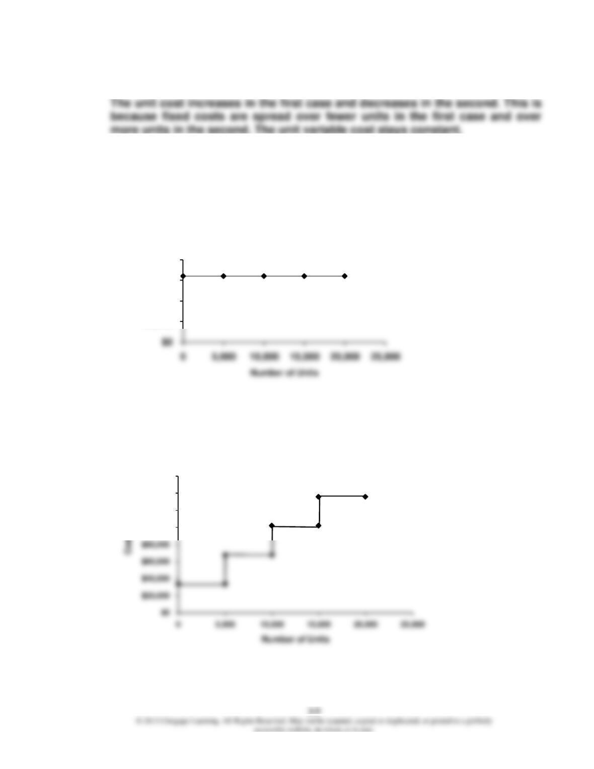
8. a. and b. 19,500 Units 21,600 Units

Unit costa $29.19* $26.48

Unit fixed costb 27.85* 25.14

Exercise 3.10 (Concluded)

Exercise 3.11

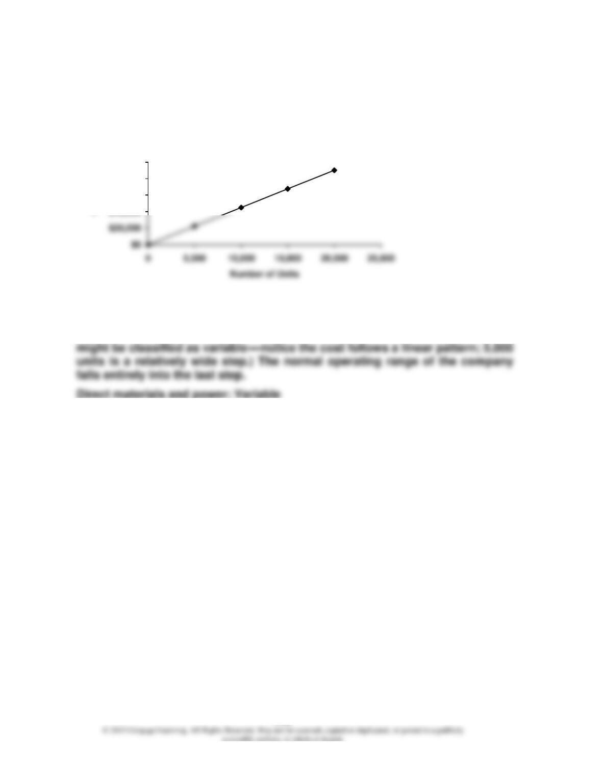
1. a. Graph of equipment depreciation:

Equipment Depreciation

$5,000

$10,000

$15,000

$20,000

Cost

b. Graph of supervisors’ wages:

Supervisors’ Wages

$100,000

$120,000

$140,000

$160,000

3-10

Exercise 3.11 (Concluded)

c. Graph of direct materials and power:

Direct Materials and Power

$40,000

$60,000

$80,000

$100,000

Cost

2. Equipment depreciation: Fixed

Supervisors’ wages: Fixed (Although if the step were small enough, the cost

Exercise 3.12

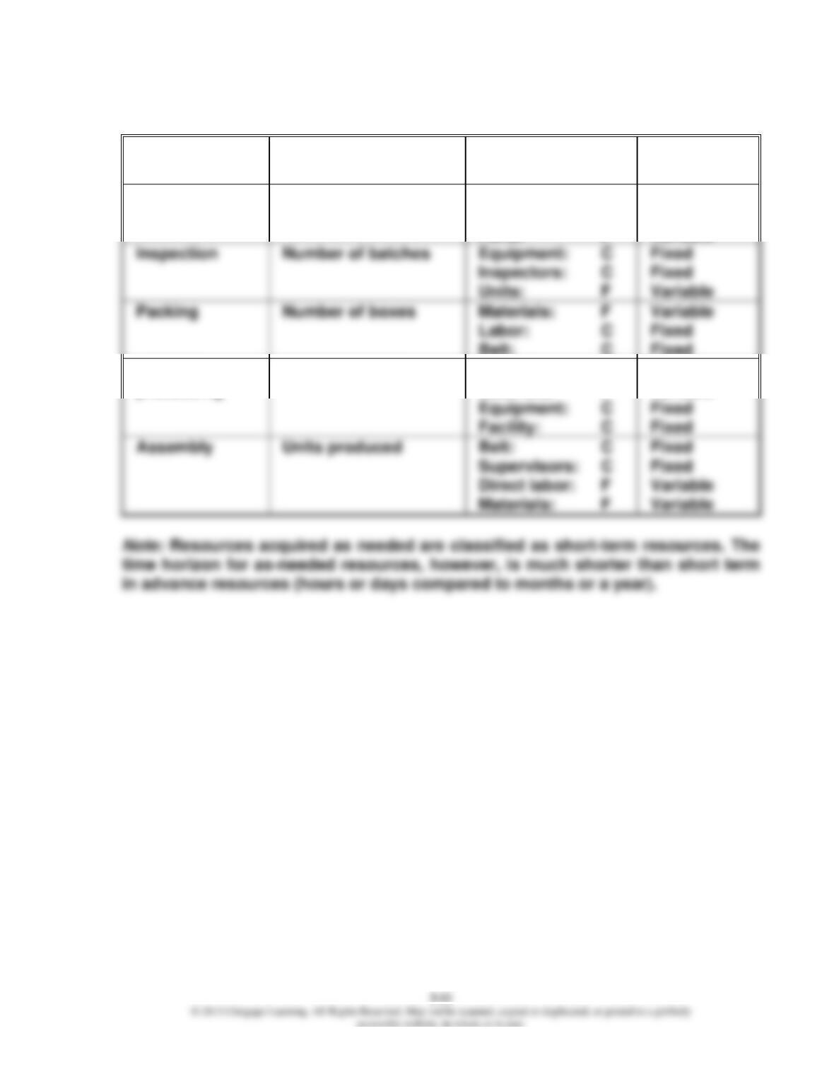
Activity

Cost Driver

Flexible (F) or

Committed (C)

Variable

or Fixed

Maintenance

Maintenance hours

Equipment: C

Labor: C

Parts: F

Fixed

Variable

Inspection

Number of batches

Equipment: C

Inspectors: C

Units: F

Fixed

Variable

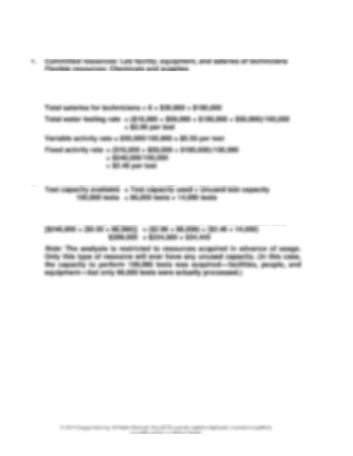
Belt: C

Fixed

Payable

processing

Number of bills

Assembly

Units produced

Belt: C

Fixed

Clerks: C

Materials: F

Fixed

Variable

3-12

Exercise 3.13

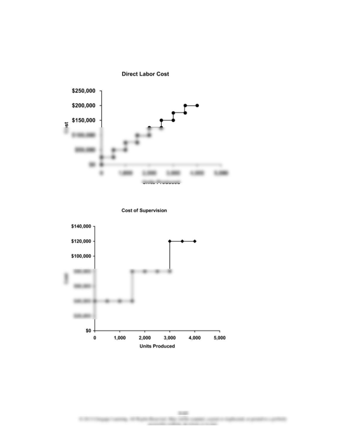
2. Depreciation on lab facility = $160,000/10 = $16,000

Depreciation on equipment = $250,000/5 = $50,000

3. Activity availability = Activity usage + Unused activity

4. Cost of activity supplied = Cost of activity used + Cost of unused activity

Cost of activity supplied = Cost of 86,000 tests + Cost of 14,000 tests

Exercise 3.14

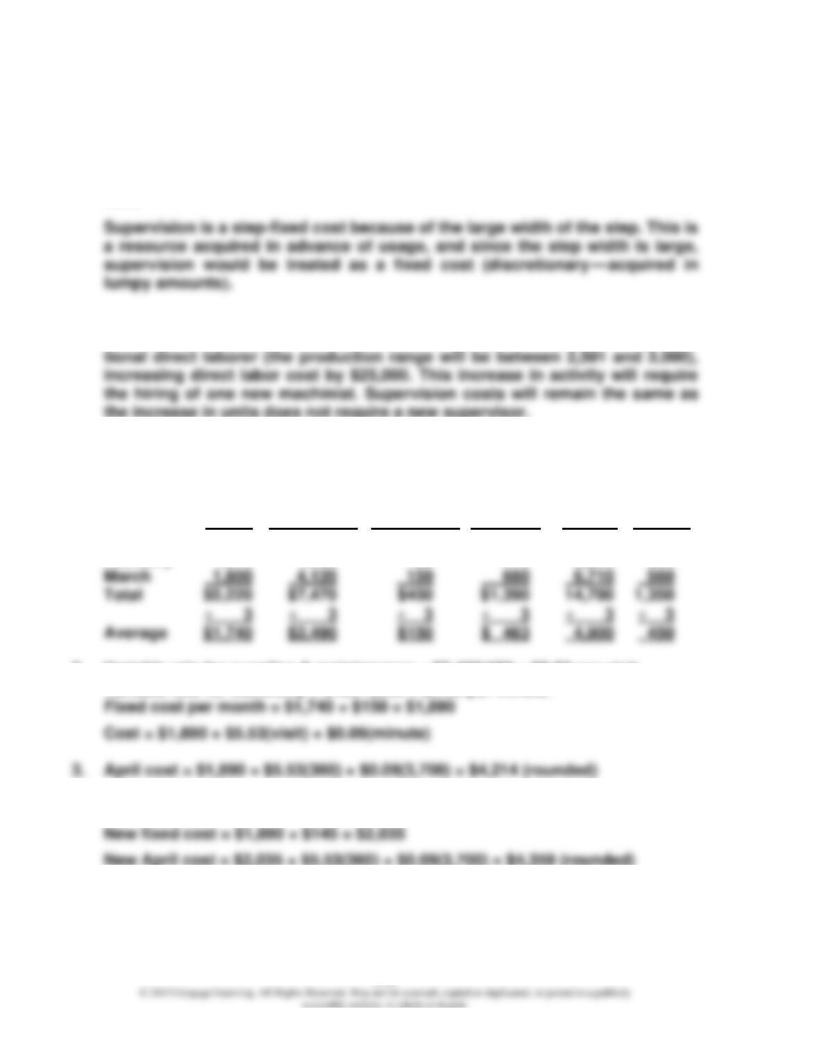
1. a. Graph of direct labor cost:

b. Graph of cost of supervision:

3-14

Exercise 3.14 (Concluded)

2. Direct labor cost is a step-variable cost because of the small width of the

step. The steps are small enough that we might be willing to view the re-

source as one acquired as needed and, thus, treated simply as a variable

cost.

3. Currently, direct labor cost is $125,000 (in the 2,001 to 2,500 range). If produc-

tion increases by 400 units next year, the company will need to hire one addi-

Exercise 3.15

1. Supplies & Equipment Tanning Number

Wages Maintenance Depreciation Electricity Minutes of Visits

January $1,750 $1,450 $150 $ 300 4,100 410

February 1,670 1,900 150 410 3,890 380

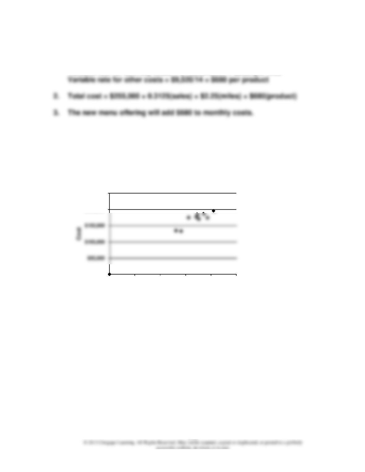
2. Variable rate for supplies & maintenance = $2,490/450 = $5.53 per visit

Variable rate for electricity = $463/4,900 = $0.09 per minute

4. Monthly depreciation on new tanning bed = [($6,960 – 0)/4]/12 = $145

3-15

Exercise 3.16

1. Variable rate for food and wages = $175,000/$560,000 = 0.3125 or 31.25%

Variable rate for delivery costs = $18,000/8,000 = $2.25 per mile

Exercise 3.17

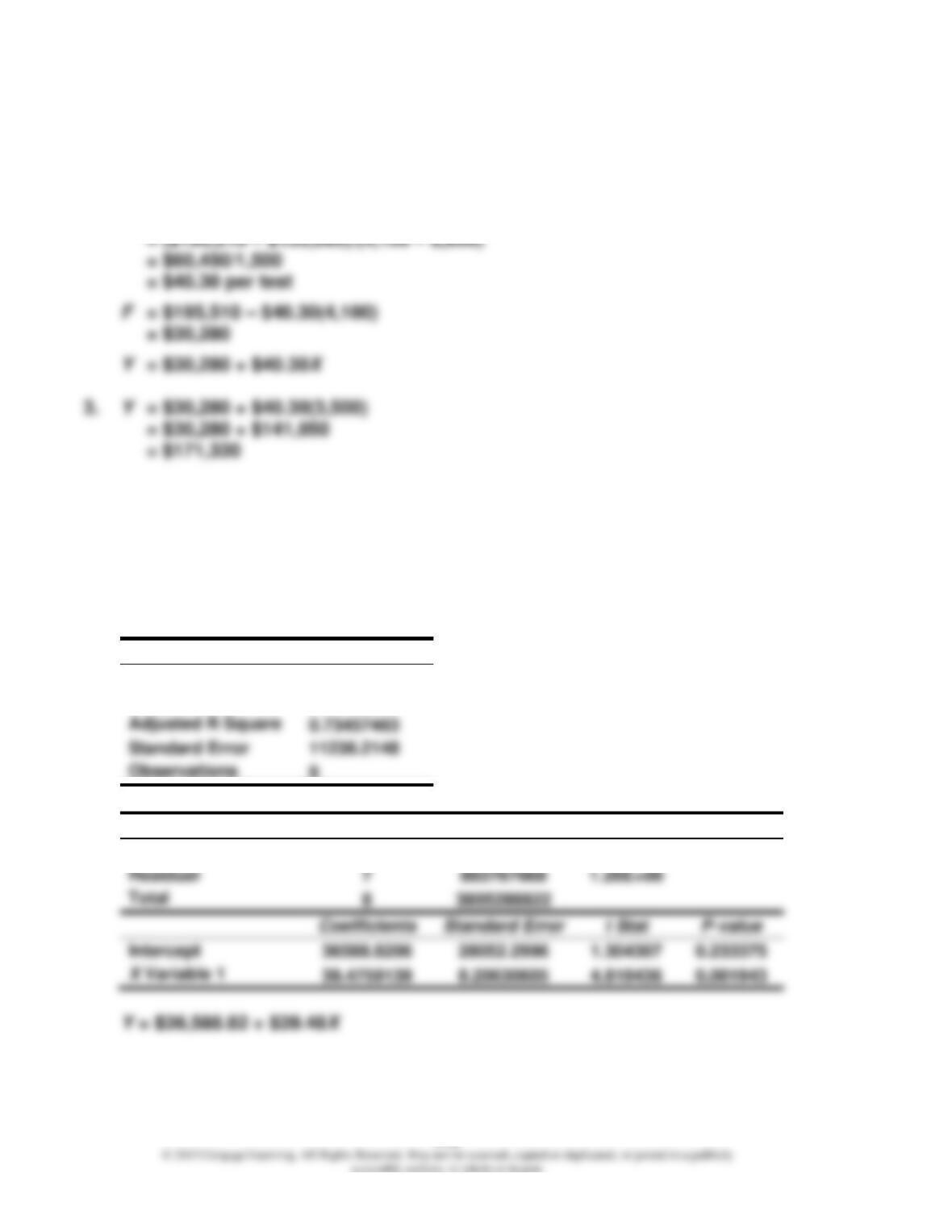
1. Scattergraph:

Scattergraph of Radiology Tests

$0

$200,000

$250,000

0 1,000 2,000 3,000 4,000 5,000

Number of Tests

Yes, there appears to be a linear relationship.

3-16

Exercise 3.17 (Concluded)

2. Low: 2,600, $135,060

High: 4,100, $195,510

V = (Y2 – Y1)/(X2 – X1)

Exercise 3.18

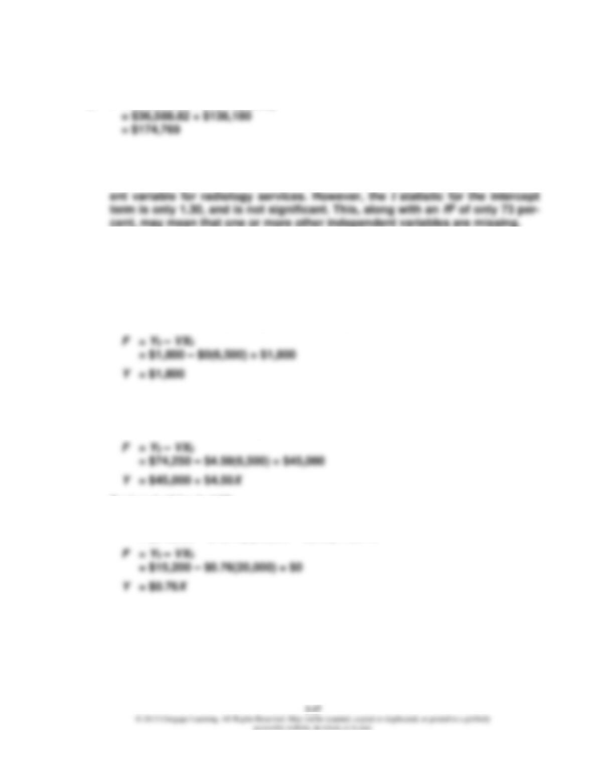
1. Regression output from spreadsheet:

SUMMARY OUTPUT

Regression Statistics

Multiple R

0.87621504

R Square

0.7677528

Adjusted R Square

0.73457463

Standard Error

11236.2148

Observations

9

ANOVA

df

SS

MS

F

Regression

1

2921521154

2.92E+09

23.1403

Residual

7

Total

8

3805288822

Intercept

Exercise 3.18 (Concluded)

2. Y = $36,588.82 + $39.48(3,500)

3. R2 is about 0.73, meaning that about 73 percent of the variability in the radiol-

ogy services cost is explained by the number of tests. The t statistic for X is

4.81 and is significant, meaning that the number of tests is a good independ-

Exercise 3.19

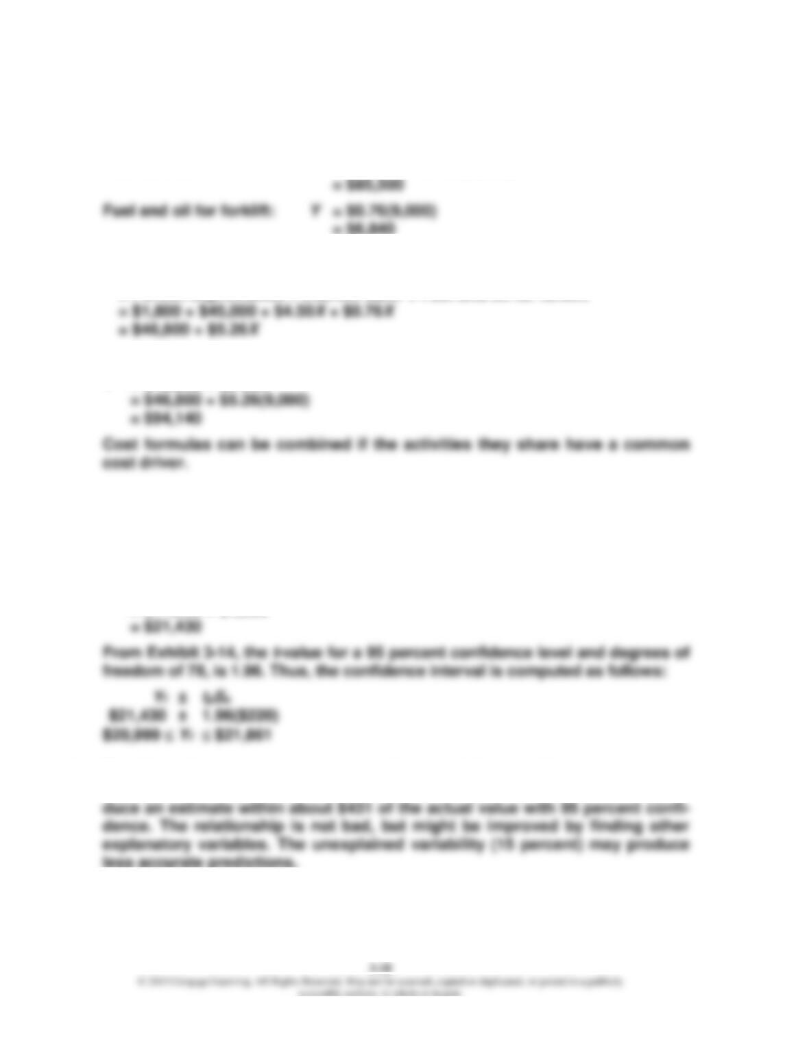
1. Forklift depreciation:

V = (Y2 – Y1)/(X2 – X1)

= ($1,800 – $1,800)/(20,000 – 6,500) = $0

Indirect labor:

V = (Y2 – Y1)/(X2 – X1)

= ($135,000 – $74,250)/(20,000 – 6,500) = $4.50

Fuel and oil for forklift:

V = (Y2 – Y1)/(X2 – X1)

= ($15,200 – $4,940)/(20,000 – 6,500) = $0.76

Exercise 3.19 (Concluded)

2. Forklift depreciation: Y = $1,800

Indirect labor: Y = $45,000 + $4.50(9,000)

3. Materials handling cost:

= Forklift depreciation + Indirect labor + Fuel and oil for forklift

For 9,000 purchase orders:

Y = $46,800 + $5.26X

Exercise 3.20

1. Y = $17,350 + $12X

2. Y = $17,350 + $12(340)

= $17,350 + $4,080

3. To obtain the percentage explained, the correlation coefficient needs to be

squared: 0.92 × 0.92 = 0.8464 or 84.64 percent. The standard error will pro-

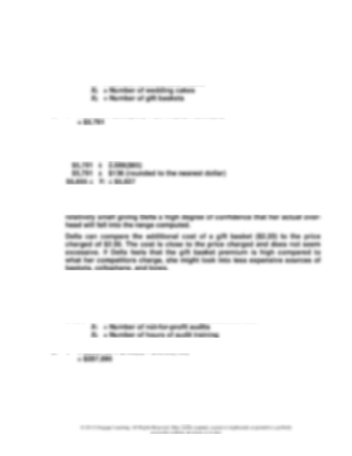
3-19

Exercise 3.21

1. Y = $1,980 + $2.56X1 + $67.40X2 + $2.20X3

where Y = Total overhead cost

X1 = Number of direct labor hours

2. Y = $1,980 + $2.56(550) + $67.40(35) + $2.20(20)

3. The t-value for a 95 percent confidence interval and 20 (24 observations – 4

variables) degrees of freedom is 2.086 (see Exhibit 3-14).

Yf ± tpSe

4. In this equation, the independent variables explain 92 percent of the variabil-

ity in overhead costs. Overall, the equation is good. R2 is high; the t-values

for all independent variables are quite high; and the confidence interval is

Exercise 3.22

1. Y = $286,700 + $790X1 – $45.50X2

where Y = Total monthly cost of audit professional time

2. Y = $286,700 + $790(9) – $45.50(130)

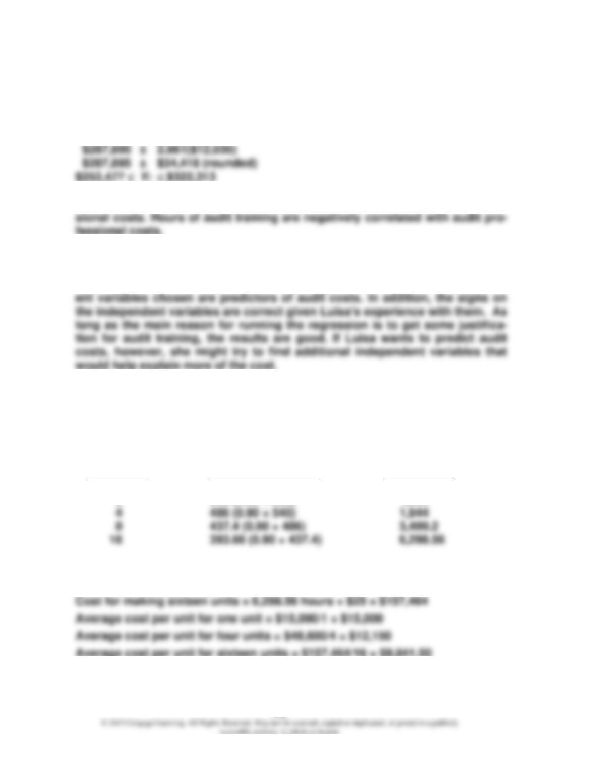
3-20

Exercise 3.22 (Concluded)

3. The t-value for a 99 percent confidence interval and degrees of freedom of 19

is 2.861 (see Exhibit 3-14).

Yf ± tpSe

4. The number of not-for-profit audits is positively correlated with audit profes-

5. In this equation, the independent variables explain 79 percent of the variabil-

ity in audit costs. Overall, the equation is not bad. The confidence interval is

relatively wide; however, the t-values are high, indicating that the independ-

Exercise 3.23

1. Cumulative Cumulative Cumulative

Number Average Time Total Time:

of Units per Unit in Hours Labor Hours

(column 1) (column 2) (3) = (1) × (2)

1 600 600

2 540 (0.90 × 600) 1,080

2. Cost for making one unit = 600 hours × $25 = $15,000

Cost for making four units = 1,944 hours × $25 = $48,600