3-62 (continued).
e. $10,510,800
Target volume in units
=
Fixed costs + [Target profit ÷ (1 − t)]
Unit contribution margin
=
$1,800,000 + [$2,843,750 ÷ (1 − .35)]
$235
=
$1,800,000 + $4,375,000
$235
=
26,277 units (rounded)
Sales dollars
=
$10,510,800 (= 26,277 $400)
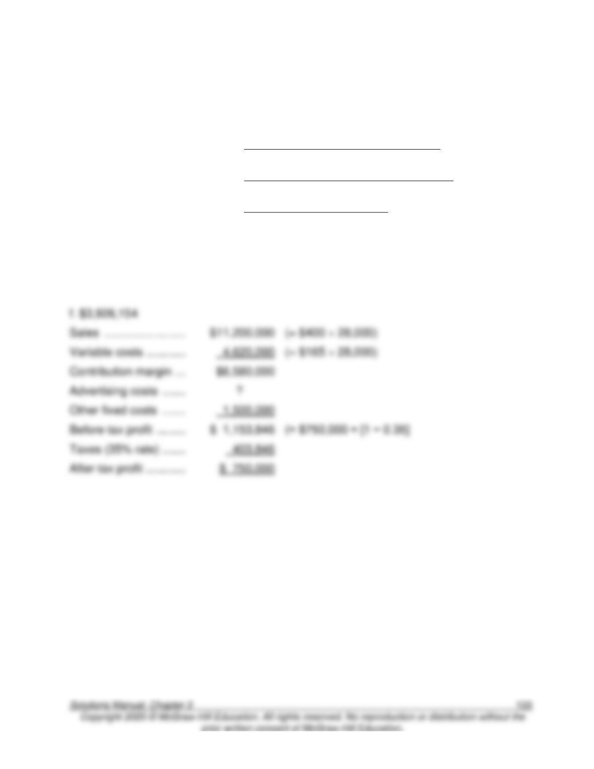
(= $750,000 ÷ [1 − 0.35]
To find the maximum advertising cost to maintain after-tax profit of $750,000, solve as
follows:
Contribution Margin ($6,580,000) – Advertising Costs – Other Fixed Costs
($1,500,000)
= Before-Tax Profits ($1,153,846)
$6,580,000 – $1,500,000 – $1,153,846 = Advertising Costs
Maximum Advertising Costs = $3,926,154
3-63. (30 min.) Extensions of the CVP Model—Multiple Products: On-the Go, Inc.
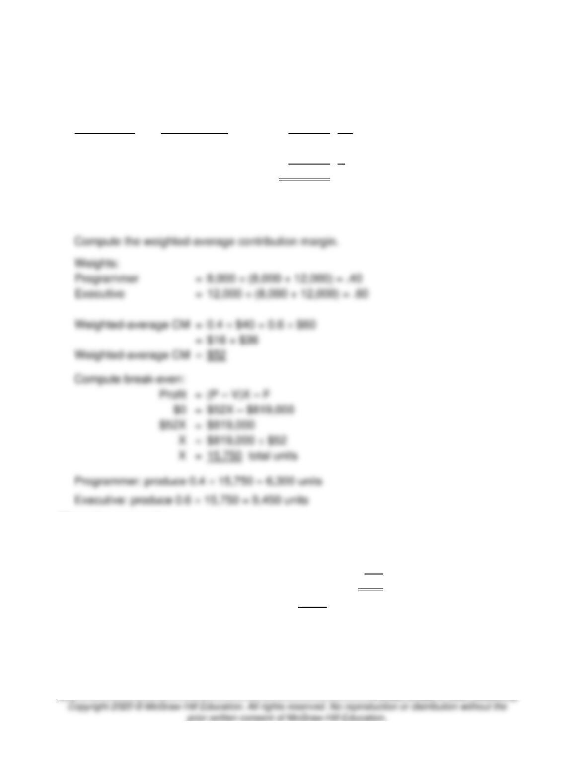
a.
Programmer
+
Executive
8,000 $70
+
12,000 $100
=
$1,760,000
PX
8,000 $30
+
12,000 $40
=
720,000
VX
8,000 $40
+
12,000 $60
=
$ 1,040,000
(P – V)X
819,000
F
$ 221,000
Profit
b.
Weights:
Programmer
=
8,000 ÷ (8,000 + 12,000) = .40
Executive
=
12,000 ÷ (8,000 + 12,000) = .60
Weighted-average CM
=
0.4 $40 + 0.6 $60
=
=
=
$819,000
=
$819,000 ÷ $52
Alternative approach:
Define a package containing 4 Programmer and 6 Executive models:
Price
4 $70 + 6 $100 =
$880
Variable cost
4 $30 + 6 $40 =
360
Contribution margin
$520
Break-even
$819,000 ÷ $520 =
1,575 packages
Programmer model:
4 1,575 packages =
6,300 units
Executive model:
6 1,575 packages =
9,450 units
3-63. (continued).
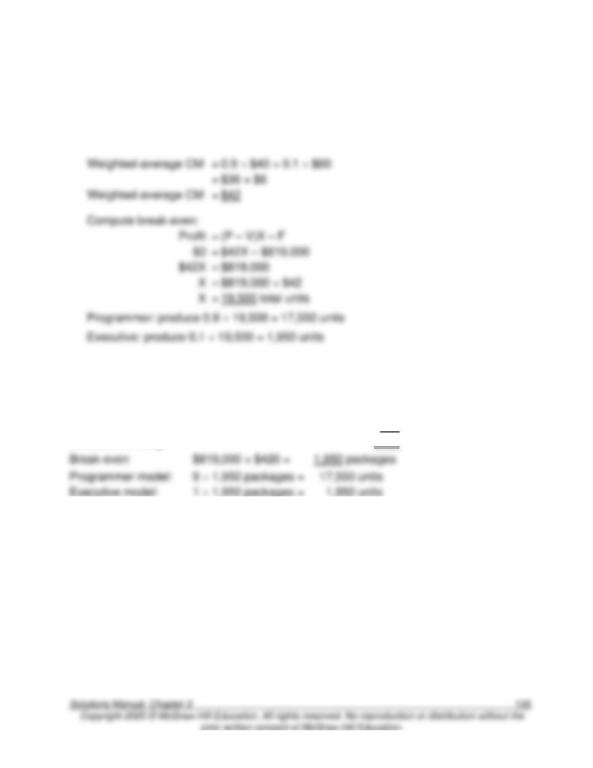
c. New weights:
Weights:
Programmer
=
.90
Executive
=
.10
Weighted-average CM
=
0.9 $40 + 0.1 $60
=
=
=
=
$819,000
=
$819,000 ÷ $42
=
19,500 total units
Alternative approach:
Define a package containing 9 Programmer and 1 Executive models:
Price
9 $70 + 1 $100 =
$730
Variable cost
9 $30 + 1 $40 =
310
Contribution margin
$420
Break-even
$819,000 ÷ $420 =
1,950 packages
Programmer model:
9 1,950 packages =
Executive model:
1 1,950 packages =
3-64. (30 min.) Extensions of the CVP Model—Multiple Products: Sundial, Inc.
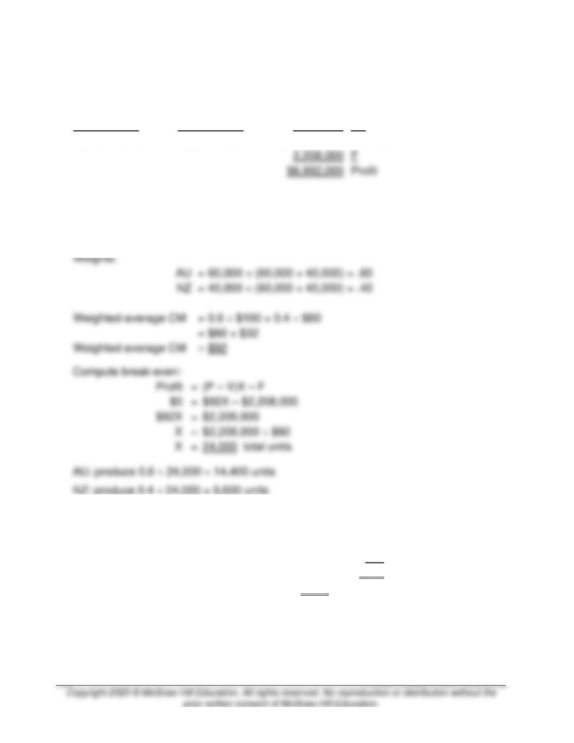
a.
AU
+
NZ
60,000 $160
+
40,000 $160
=
$16,000,000
PX
60,000 $60
+
40,000 $80
=
6,800,000
VX
60,000 $100
+
40,000 $80
=
$ 9,200,000
(P – V)X
F
b.
Compute the weighted-average contribution margin.
Weights:
60,000 ÷ (60,000 + 40,000) = .60
40,000 ÷ (60,000 + 40,000) = .40
Weighted-average CM
0.6 $100 + 0.4 $80
$60 + $32
=
=
$2,208,000
=
$2,208,000 ÷ $92
Alternative approach:
Define a package containing 6 AU and 4 NZ models:
Price
6 $160 + 4 $160 =
$1,600
Variable cost
6 $60 + 4 $80 =
680
Contribution margin
$920
Break-even
$2,208,000 ÷ $920 =
2,400 packages
AU model:
6 2,400 packages =
14,400 units
NZ model:
4 2,400 packages =
9,600 units
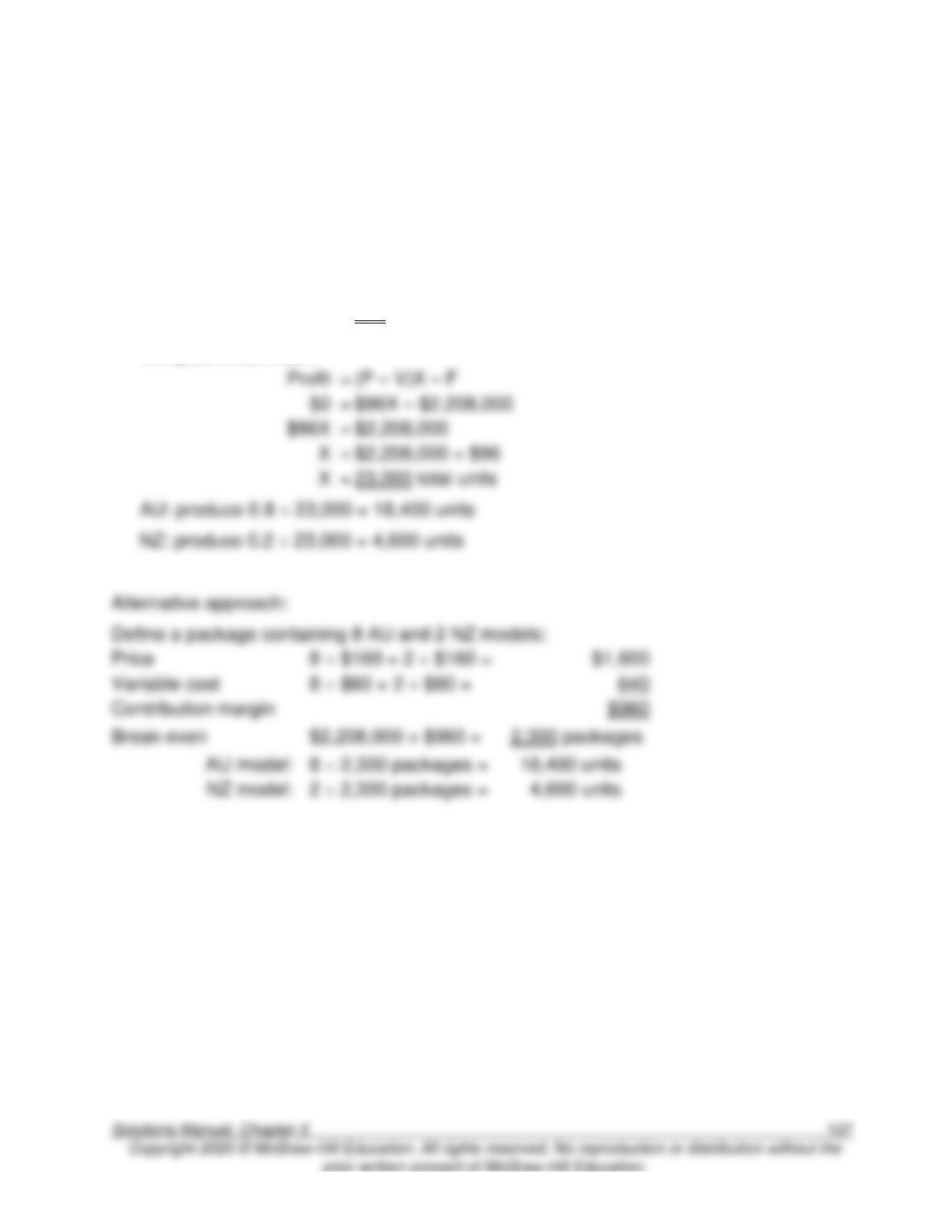
3-64. (continued).
c. New weights:
Weights:
AU
=
.80
NZ
=
.20
Weighted-average CM
=
0.8 $100 + 0.2 $80
=
$80 + $16
Weighted-average CM
=
$96
Compute break-even:
=
=
=
$2,208,000
=
$2,208,000 ÷ $96
=
23,000 total units
Variable cost
3-65. (30 min.) Extensions of the CVP Model—Multiple Products: Sell Block.
a.
Individuals
+
Partnerships
+
Corporations
60,000 $200
+
4,000 $1,000
+
16,000 $2,000
=
$48,000,000
PX
60,000 $180
+
4,000 $900
+
16,000 $1,800
=
43,200,000
VX
60,000 $20
+
4,000 $100
+
16,000 $200
=
$ 4,800,000
(P – V)X
3,690,000
F
$ 1,110,000
Profit
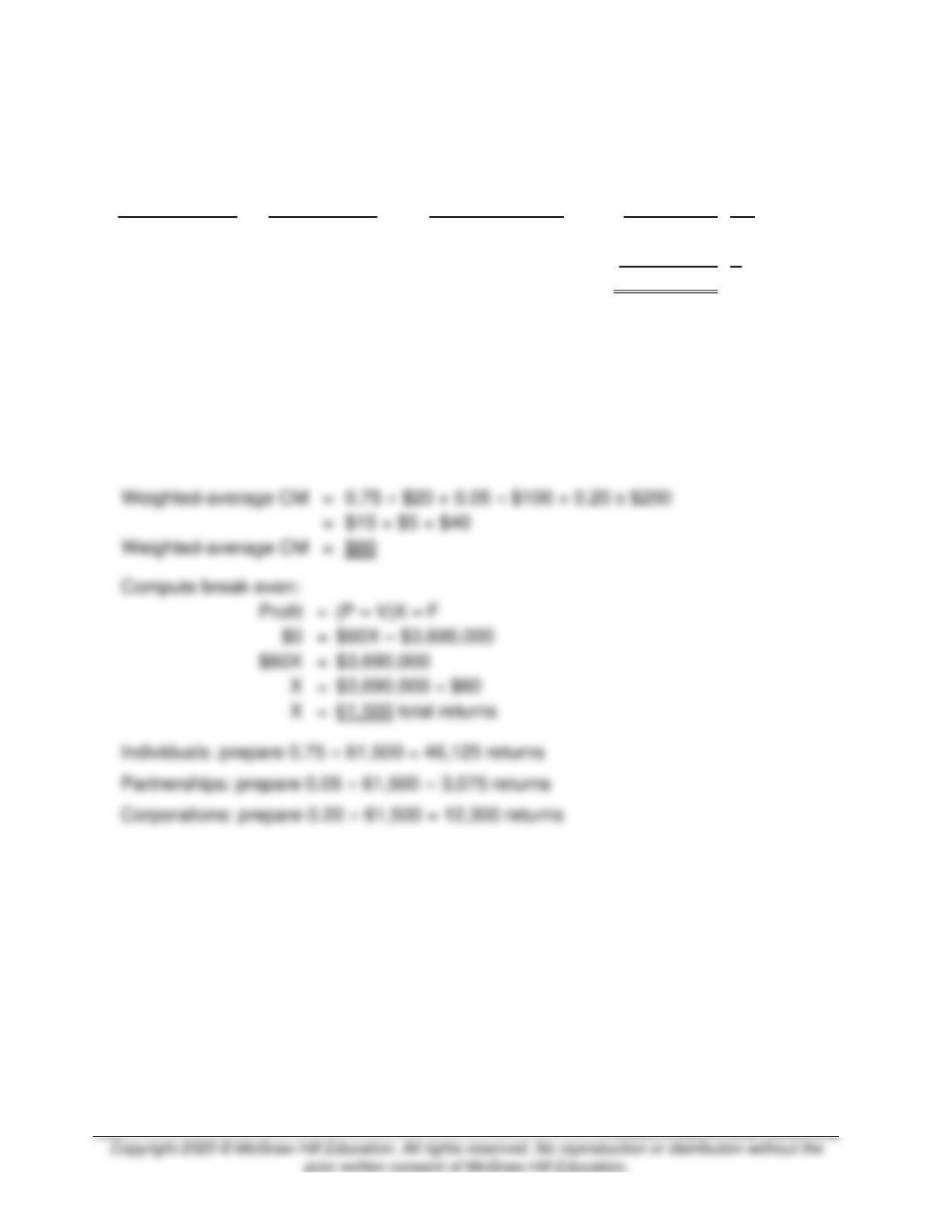
b. Compute the weighted-average contribution margin.
Weights:
Individuals
=
60,000 ÷ (60,000 + 4,000 + 16,000) = .75
Partnerships
=
4,000 ÷ (60,000 + 4,000 + 16,000) = .05
Corporations
=
16,000 ÷ (60,000 + 4,000 + 16,000) = .20
Weighted-average CM
=
0.75 $20 + 0.05 $100 + 0.20 x $200
=
$15 + $5 + $40
=
(P – V)X – F
=
=
$3,690,000
=
$3,690,000 ÷ $60
3-65. (continued).
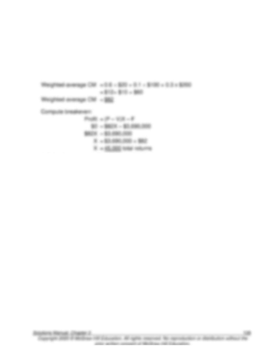
c. New weights:
Weights:
Individuals
=
.60
Partnerships
=
.10
Corporations
=
.30
Weighted-average CM
=
0.6 $20 + 0.1 $100 + 0.3 x $200
=
$12+ $10 + $60
=
=
=
$3,690,000
=
$3,690,000 ÷ $82
=
45,000 total returns
Individuals: prepare 0.60 45,000 = 27,000 returns
Partnerships: prepare 0.10 45,000 = 4,500 returns
Corporations: prepare 0.30 45,000 = 13,500 returns
3-66. (20 min.) Extensions of CVP Analysis—Multiple Products: Minot Furniture.
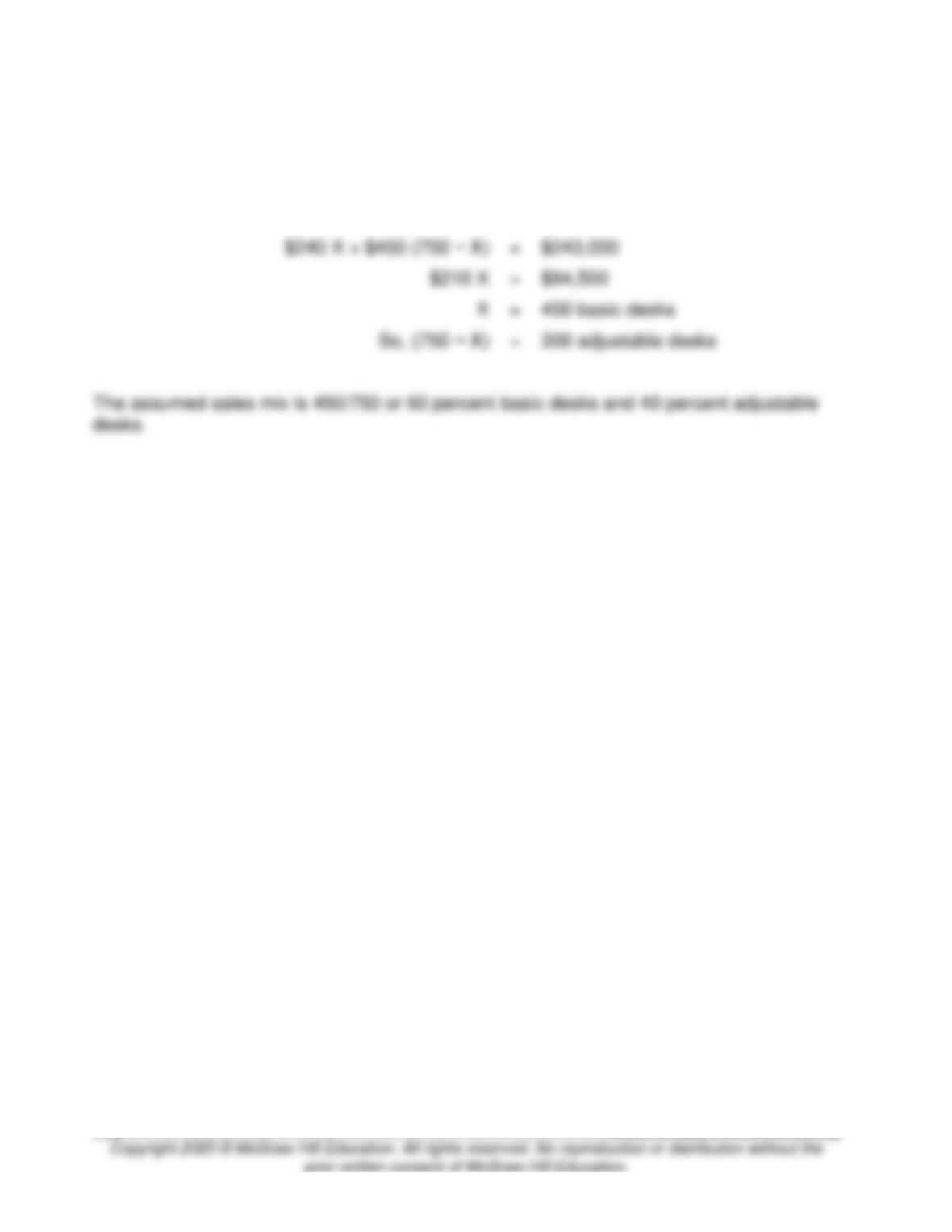
At the break-even point of 750 total units, the total contribution margin will equal the fixed
costs. Let X = the number of basic desks sold at the break-even point. Then (750 − X) will
equal the number of adjustable desks sold at the break-even point. Therefore,
($600 − $360) X + ($900 − $450) (750 − X)
=
$243,000
=
$243,000
=
=
=
3-67. (30 min.) Extensions of the CVP Basic Model—Multiple Products and Taxes:
Ocean King Products.
a. Compute weighted-average contribution margins for each product.
Weights
Selling
Price per
case
Variable
Cost per
Case
Contribution
Margin per
Case
Variety 1
.40
$ 3
$ 2
$1
Variety 2
.35
5
3
2
Variety 3
.25
10
6
4
Weighted-average Revenue
=
.4 $3 + .35 x $5 + .25 $10
=
$5.45
Weighted-average CM
=
.4 $1 + .35 x $2 + .25 $4
=
$2.10
Weighted-average CM%
=
$2.10 ÷ $5.45 = 38.5321% (rounded)
Compute break-even revenue:
Break-even revenue
=
F ÷ Weighted-average CM%
=
$46,200 ÷ 38.5321%
=
$119,900 (rounded)
=
=
=
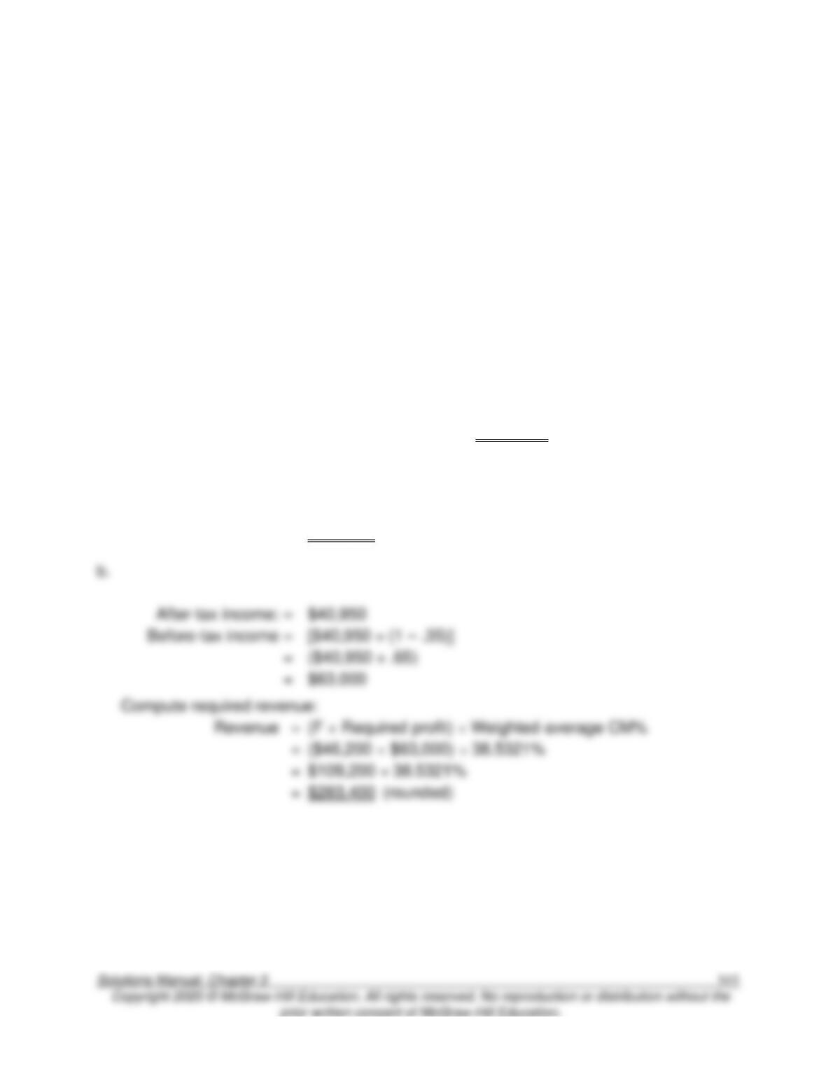
($40,950 ÷ .65)
=
=
(F + Required profit) ÷ Weighted-average CM%
=
($46,200 + $63,000) ÷ 38.5321%
=
$109,200 ÷ 38.5321%
3-68. (30 min.) Extensions of the CVP Model—Multiple Products and Taxes:
Limitless Labs, Inc.
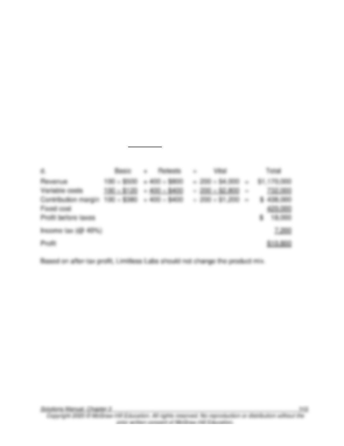
a.
Basic
+
Retest
+
Vital
Total
Revenue
850 $500
+
100 $800
+
50 $4,000
=
$705,000
Variable costs
850 $120
+
100 $400
+
50 $2,800
=
282,000
Contribution margin
850 $380
+
100 $400
+
50 $1,200
=
$ 423,000
Fixed cost
390,000
Profit before taxes
$ 33,000
Income tax (@ 40%)
13,200
Profit
$19,800
b. Compute weighted-average contribution margin percentages for each product.
Basic
Retest
Vital
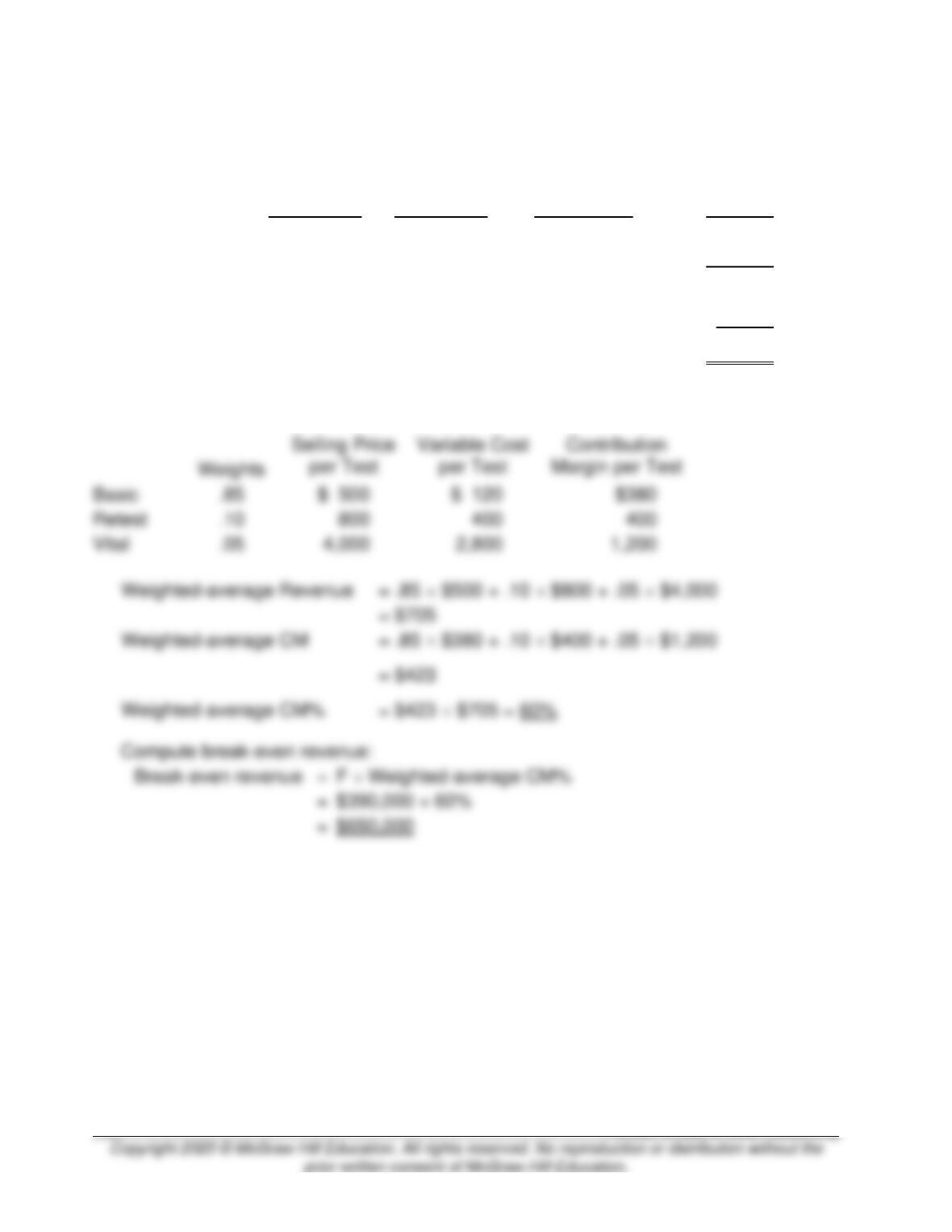
Weighted-average Revenue
=
.85 $500 + .10 $800 + .05 $4,000
=
$705
=
F ÷ Weighted-average CM%
=
$390,000 ÷ 60%
3-68. (continued).
c.
After-tax income:
=
$180,000
Before-tax income
=
[$180,000 ÷ (1 – .40)]
=
($180,000 ÷ .60)
=
$300,000
Compute required revenue:
Revenue
=
(F + Required profit) ÷ Weighted-average CM%
=
($390,000 + $300,000) ÷ 60%
=
$690,000 ÷ 60%
=
$1,150,000
Revenue
+
Variable costs
+
Contribution margin
+
Fixed cost
3-69. (30 min.) Extensions of the CVP Model—Multiple Products and Taxes:
Painless Dental Clinics, Inc.
a.
Cleaning
+
Filling
+
Capping
Total
Revenue
9,000 $120
+
900 $400
+
100 $1,200
=
$1,560,000
Variable costs
9,000 $80
+
900 $300
+
100 $500
=
1,040,000
Contribution margin
9,000 $40
+
900 $100
+
100 $700
=
$ 520,000
Fixed cost
400,000
Profit before taxes
$ 120,000
Income tax (@ 30%)
36,000
Profit
$84,000
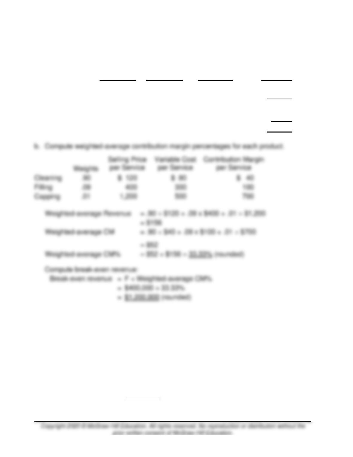
Cleaning
Filling
Capping
Weighted-average Revenue
.90 $120 + .09 x $400 + .01 $1,200
$156
=
F ÷ Weighted-average CM%
=
$400,000 ÷ 33.33%
c.
After tax income:
=
$140,000
Before tax income
=
[$140,000 ÷ (1 – .30)]
=
($140,000 ÷ .70)
=
$200,000
Compute required revenue:
Revenue
=
(F + Required profit) ÷ Weighted-average CM%
=
($400,000 + $200,000) ÷ 33.33%
=
$600,000 ÷ 33.33%
=
$1,800,000 (rounded)
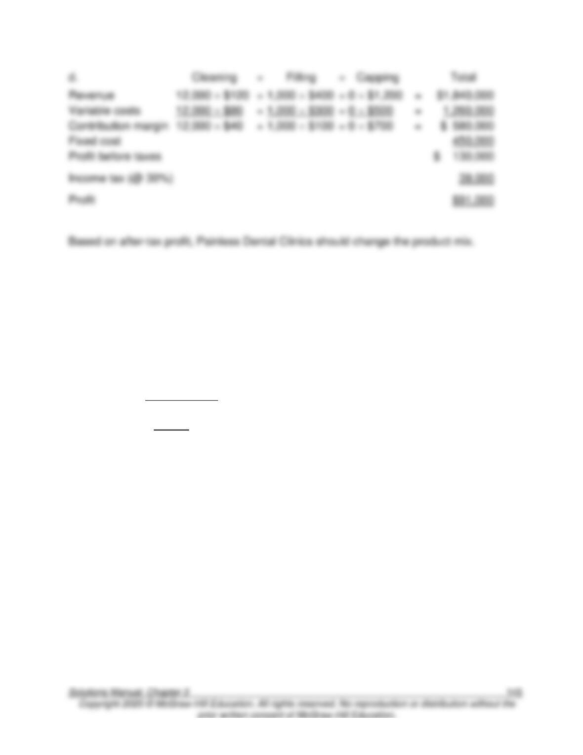
3-69. (continued).
Variable costs
1,000 $300
Contribution margin
1,000 $100
3-70. (20 min.) Extensions of the CVP Model—Taxes With Graduated Rates:
Hastings & Daughters.
a.
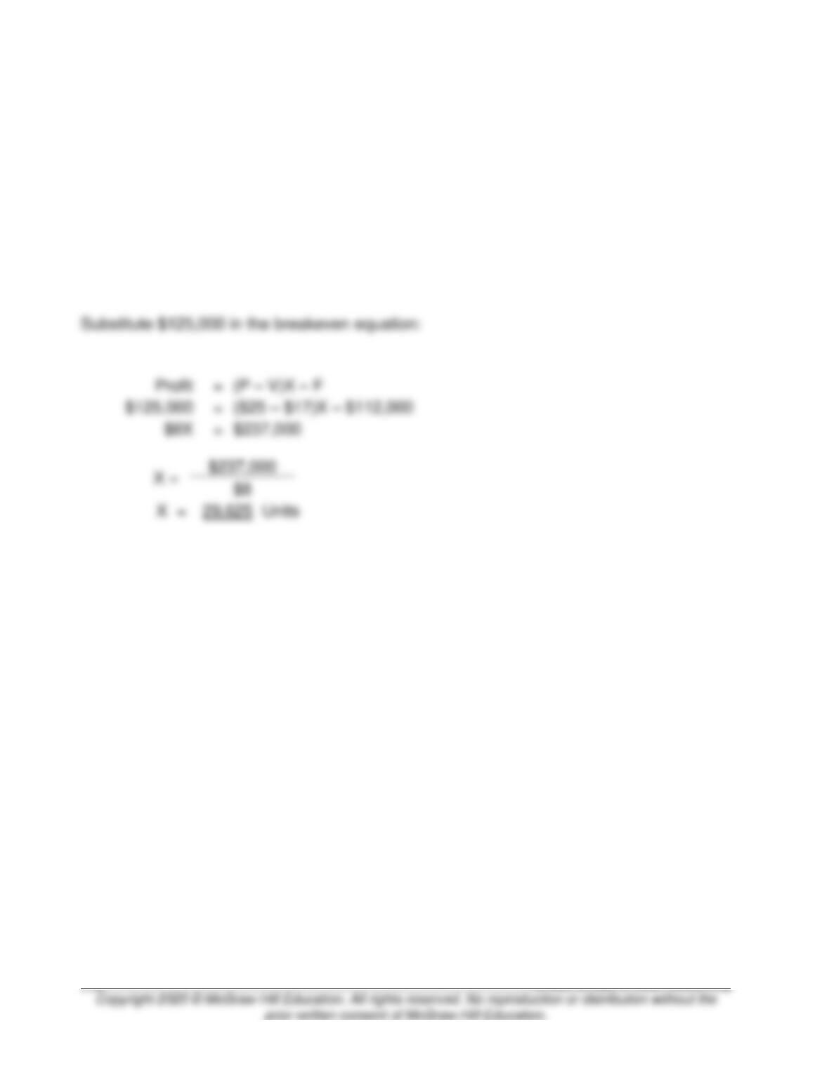
Profit
=
(P – V)X – F
$0
=
($25 – $17)X – $112,000
$8X
=
$112,000
X =
$112,000
$8
X
=
14,000
Units
3-70. (continued).
b.
First, determine the pre-tax income necessary to earn $90,000 after-tax. The first
$100,000 of income is taxed at 25 percent, so the after-tax income is $75,000:
= [100,000 (1.0 – 0.25).
To earn an additional $15,000 (= $90,000 – $75,000) after tax requires pre-tax income of
$25,000 [= $15,000 ÷ (1.0 – 0.40)]. Therefore, to earn $90,000 after tax requires pre-tax
income of $125,000 (= $100,000 + $25,000).
3-71. (20 min.) CVP Analysis with Increasing Unit Variable Costs
The purpose of this problem is to illustrate that “more realistic” cost equations and price
relations with volume can be analyzed with the approaches in the chapter (although, of
course, the simple formulas that applied when the relations were linear will not work here.)
The unit cost function is admitedly a bit contrived, but assuming the variable cost function
here is quadratic is not much more of a simpllification than assuming that unit variable
costs are constant across all volumes.
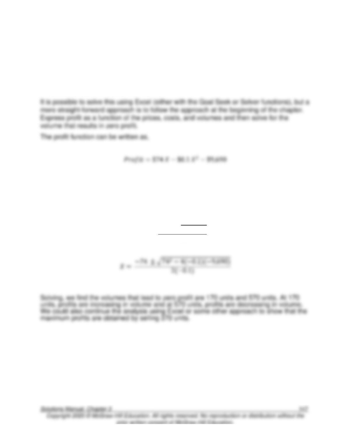
Profit is a quadratic equation and can be solved explicitly for the value of X, volume, that
results in zero profit. (It is important to note that there might be two, one, or no (real)
values of volume that lead to zero profits.
Using the quadratic formula to solve the equation where (a = -0.1, b = 74, and c = -9,690),
we find,
𝑋 = −𝑏 ± √𝑏2− 4𝑎𝑐
2𝑎
Solutions to Integrative Case
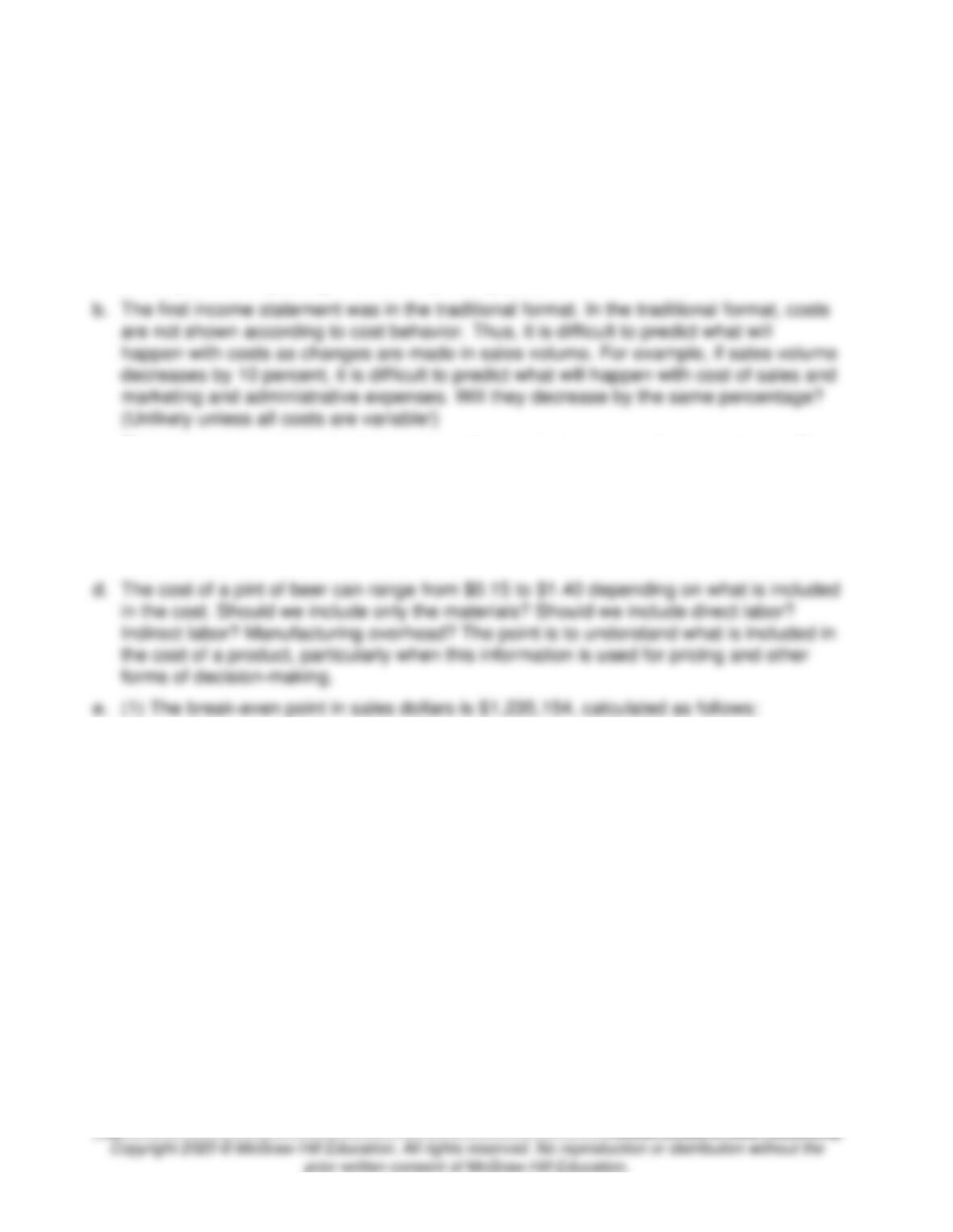
3-72. (60 min.) Financial Modeling: Roseville Brewing Company.
a. Potential investors and bankers were concerned about the accuracy of the income
statement projections. They wanted to know what would happen if the projections were
overly optimistic. Operating profit was heavily influenced by projected sales dollars and
product mix. The concern was over the impact changes in sales and product mix
(among other things) might have on operating profit.
c. The best way to quickly check for reasonableness is to compare the operating profit as
a percentage of sales to other similar businesses. In addition, the dollar amount of
operating profit can be compared to other similar businesses of roughly the same size.
(In fact, the banks and investors who were approached by RBC often looked at these
two items as a starting point to ensure the projected income statement was
reasonable.)
Breakeven point
=
Total fixed costs ÷ contribution margin ratio
=
$520,000 ÷ ($822,212 ÷ $1,953,000)
=
$520,000 ÷ .421 (rounded)
=
$1,235,154. (rounded)
(2) The margin of safety is $717,846, calculated as follows:
Margin of safety
=
$1,953,000 – $1,235,154
=
$717,846.
3-72 (continued).
(3) RBC is selling many different products that change daily. It is difficult if not
impossible, to measure units of product for a brew pub. This same argument holds true
for most service companies as well. Service companies do not sell “units” of service.
Thus, for these types of companies, break-even points and target profit points are
calculated using sales dollars.
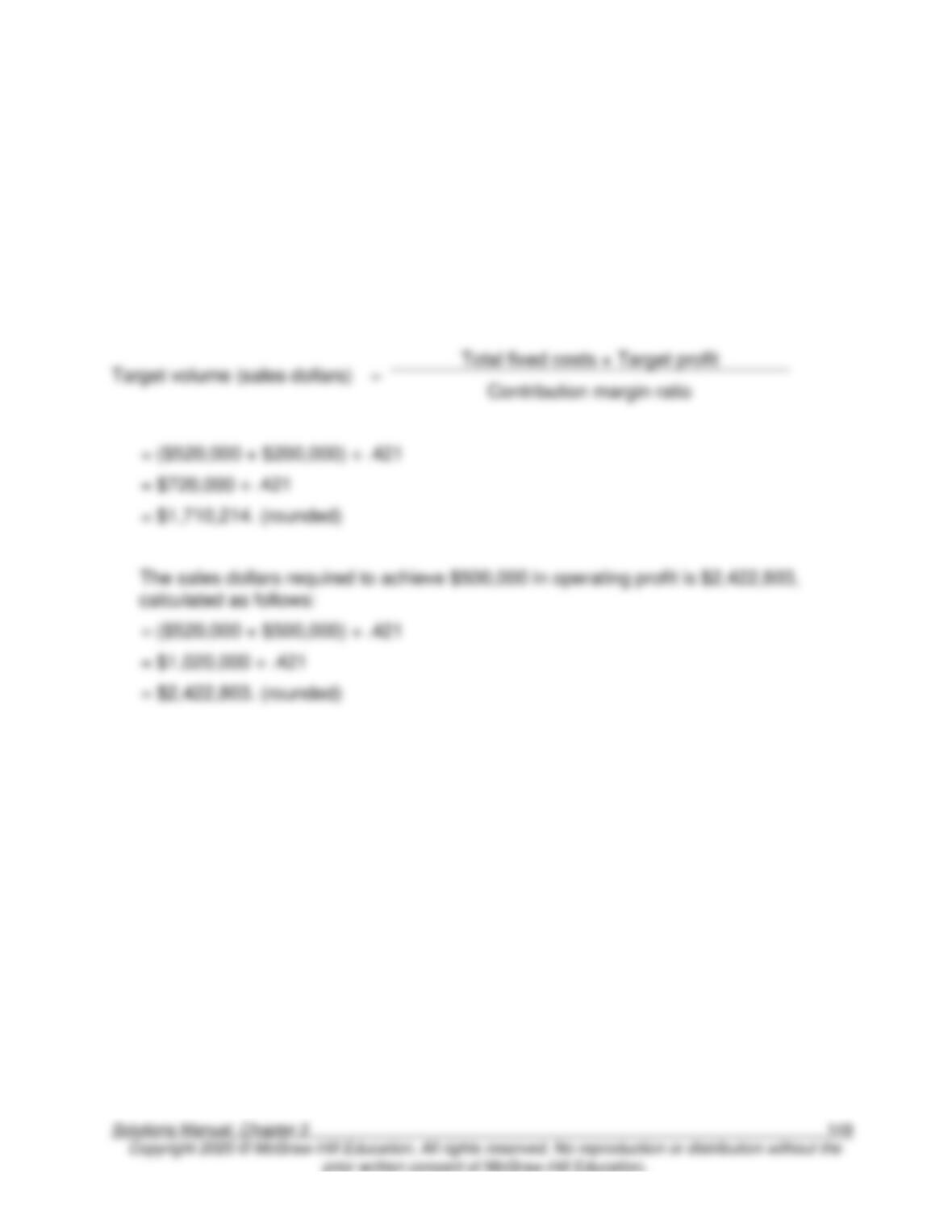
(4) The sales dollars required to achieve $200,000 in operating profit is $1,710,214,
calculated as follows:
These calculations assume that the product mix is constant. The contribution margin
ratio is dependent on the product mix, and will change as the product mix changes.