Exercise 3.23 (Concluded)
3. Cumulative Cumulative Cumulative Time
Number Average Time Total Time: for Last
of Units per Unit in Hours Labor Hours Unit
(column 1) (column 2) (1) × (2) (3) – (2)
1 600 600 600.00
2 540 1,080 480.00
5 469.79 2,348.96 404.96
7 446.37 3,124.58 382.87
Exercise 3.24
1. Cumulative Cumulative Cumulative
Number Average Time Total Time:
of Units per Unit in Hours Labor Hours
(column 1) (column 2) (3) = (1) × (2)
1 1,000 1,000
2 750 (0.75 × 1,000) 1,500
8 421.88 (0.75 × 562.5) 3,375
2. Total labor cost for eight sets = 3,375 hours × $40 = $135,000
Total labor cost for sixteen sets = 5,063 hours × $40 = $202,520
3. Cumulative Cumulative Cumulative Time
Number Average Time Total Time: for Last
of Units per Unit in Hours Labor Hours Unit
(column 1) (column 2) (1) × (2) (3) – (2)
1 1,000 1,000 1,000.00
2 750 1,500 500.00
4 562.5 2,250 348
6 475.38 2,852 288
8 421.88 3,375 254
3-22
Exercise 3.25
2. a, sales revenues
4. b, number of pairs
6. c, number of credit hours
8. d, number of orders
10. i, number of customers
3-23
CPA-TYPE EXERCISES
Exercise 3.26
d. Total contribution margin = Operating income + Fixed cost
Exercise 3.27
Exercise 3.28
Exercise 3.29
Exercise 3.30
PROBLEMS
Problem 3.31
1. Flexible resources: Direct materials, direct labor, machine operating costs
Committed resources—Long-term: Machining
Committed resources—Short-term: Purchasing, inspection, and materials
2. Total annual resource spending:
Activity Fixed Costa Variable Costb Total Cost
Material usage — $ 75,000 $ 75,000
Labor usage — 25,000 25,000
Machining $ 30,000 25,000 55,000
aMachining: lease payment of $30,000
Purchasing: 23,000 – 5,000 + 2,000 = 20,000, the required supply (demand).
Since the resource is purchased in units of 5,000, the necessary supply can
be reduced from 25,000 to 20,000. The cost of each block of resources is
3-25
Problem 3.31 (Concluded)
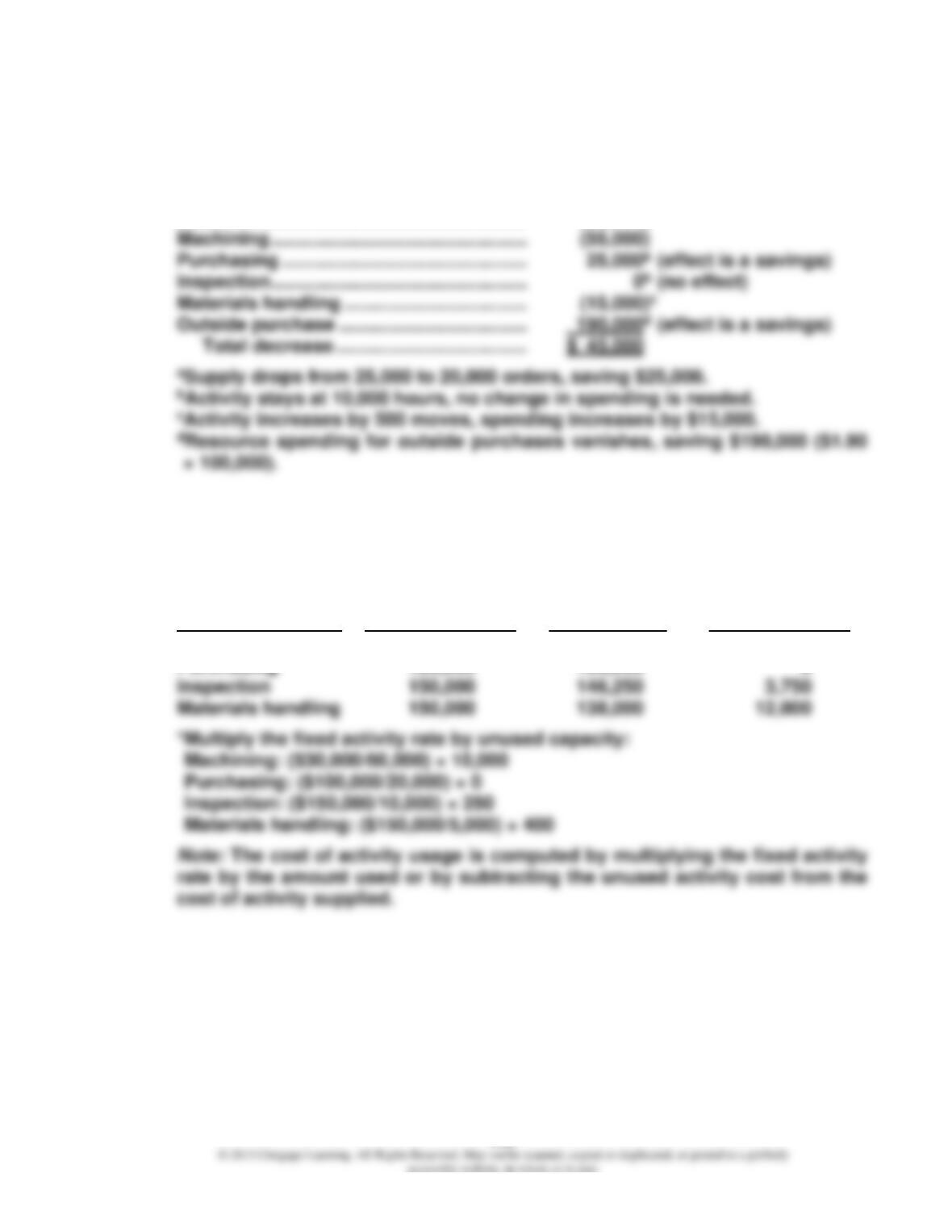
Effect on resource spending of decision to produce rollers:
Materials …………………………………………… $ (75,000)
Labor ………………………………………………… (25,000)
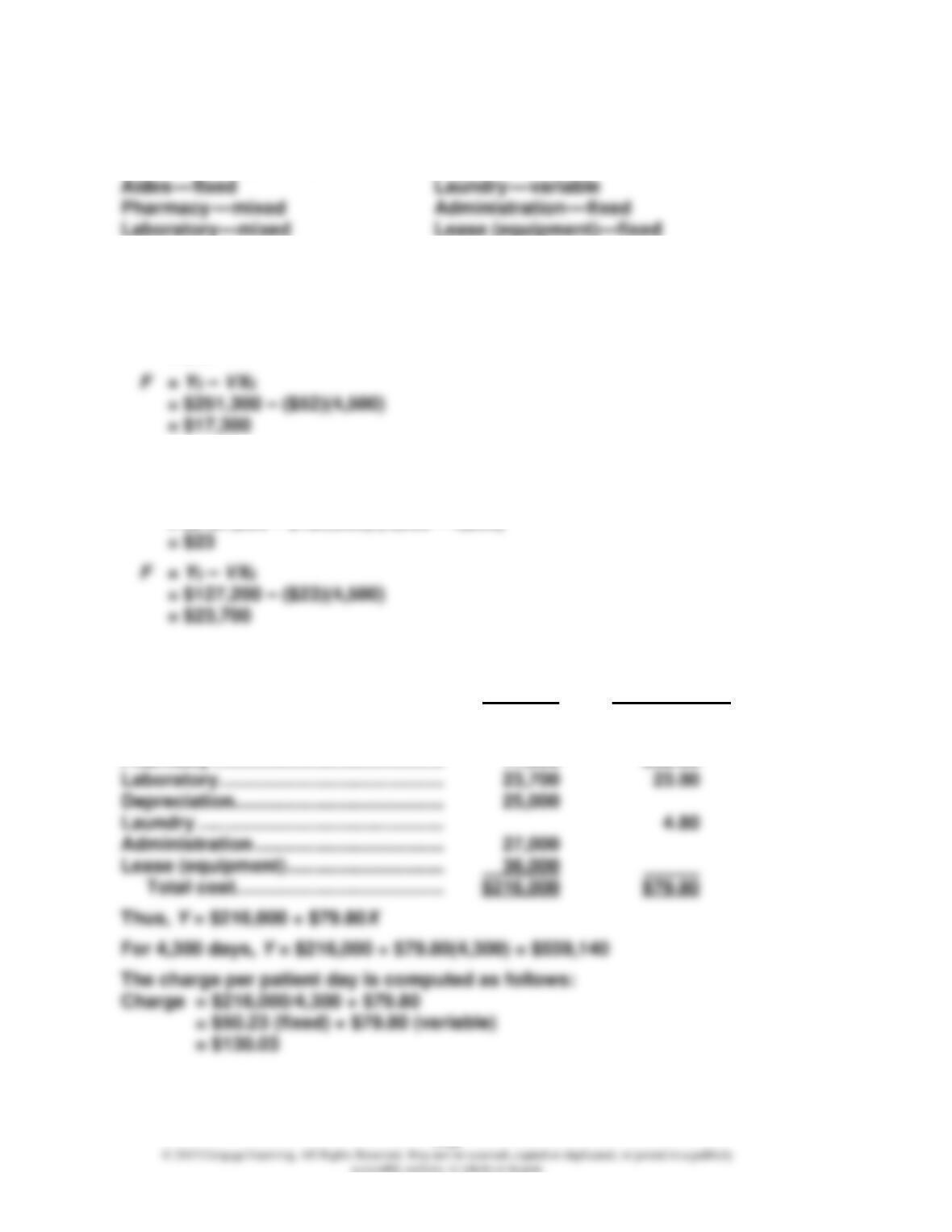
3. Materials and labor are flexible resources and have no unused capacity (Cost
of activity supplied = Cost of activity usage). Only fixed activity costs qualify
for an unused capacity component (representing committed resources). These
costs are analyzed as follows:
Cost of Cost of Cost of
Activity Activity Supplied Activity Used Unused Activity*
Machining $ 30,000 $ 25,000 $ 5,000
Purchasing 100,000 100,000 0
3-26
Problem 3.32
1. Salaries, nurses—fixed Depreciation—fixed
2. Pharmacy:
V = (Y2 – Y1)/(X2 – X1)
= ($251,300 – $235,700)/(4,500 – 4,200)
= $52
Laboratory:
V = (Y2 – Y1)/(X2 – X1)
= ($127,200 – $120,300)/(4,500 – 4,200)
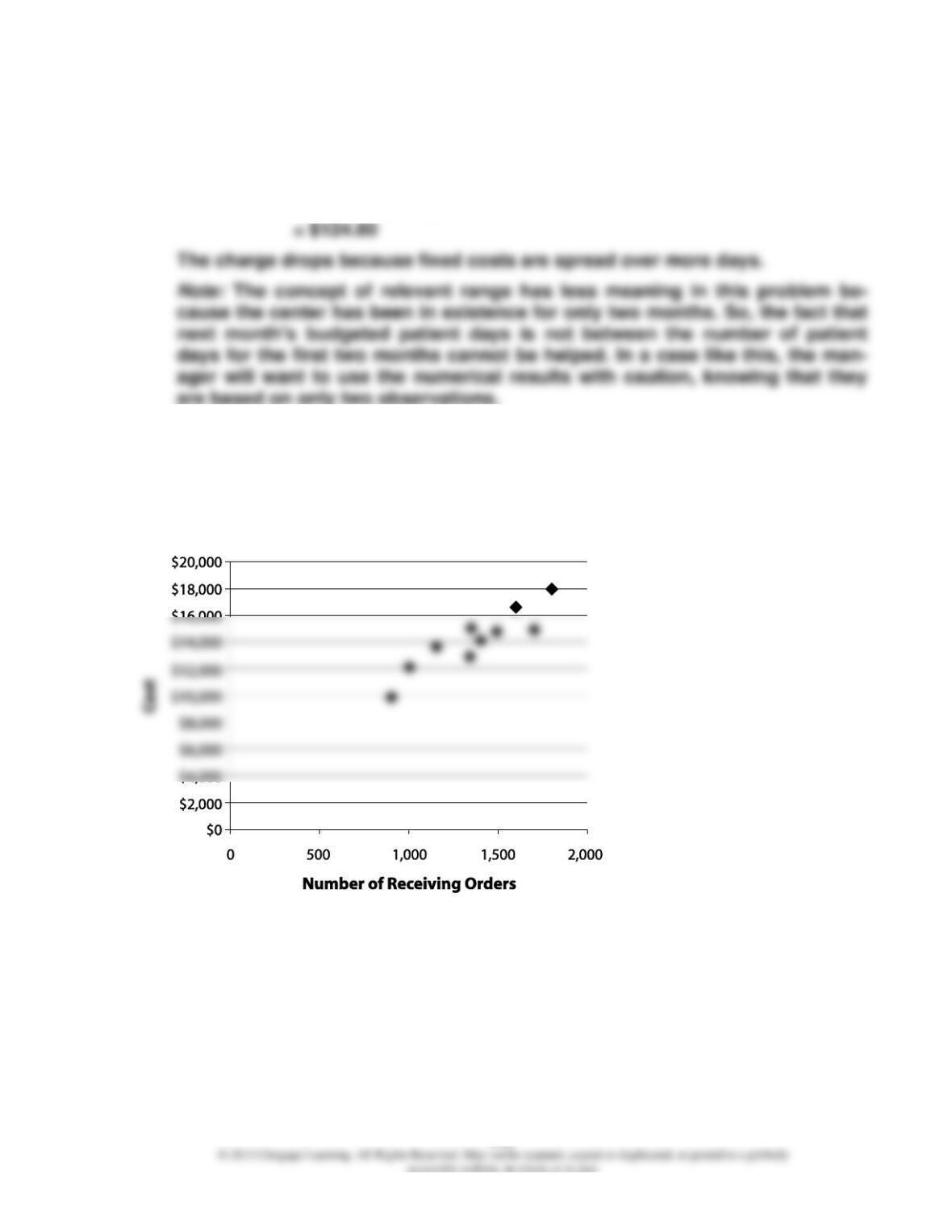
3. Unit
Fixed Variable Cost
Salaries, nurses ……………………………. $ 55,000
Aides ……………………………………………. 32,000
Pharmacy …………………………………….. 17,300 $52.00
3-27
Problem 3.32 (Concluded)
4. For 4,800 patient days:
Charge/day = $216,000/4,800 + $79.80
= $45.00 + $79.80
Problem 3.33
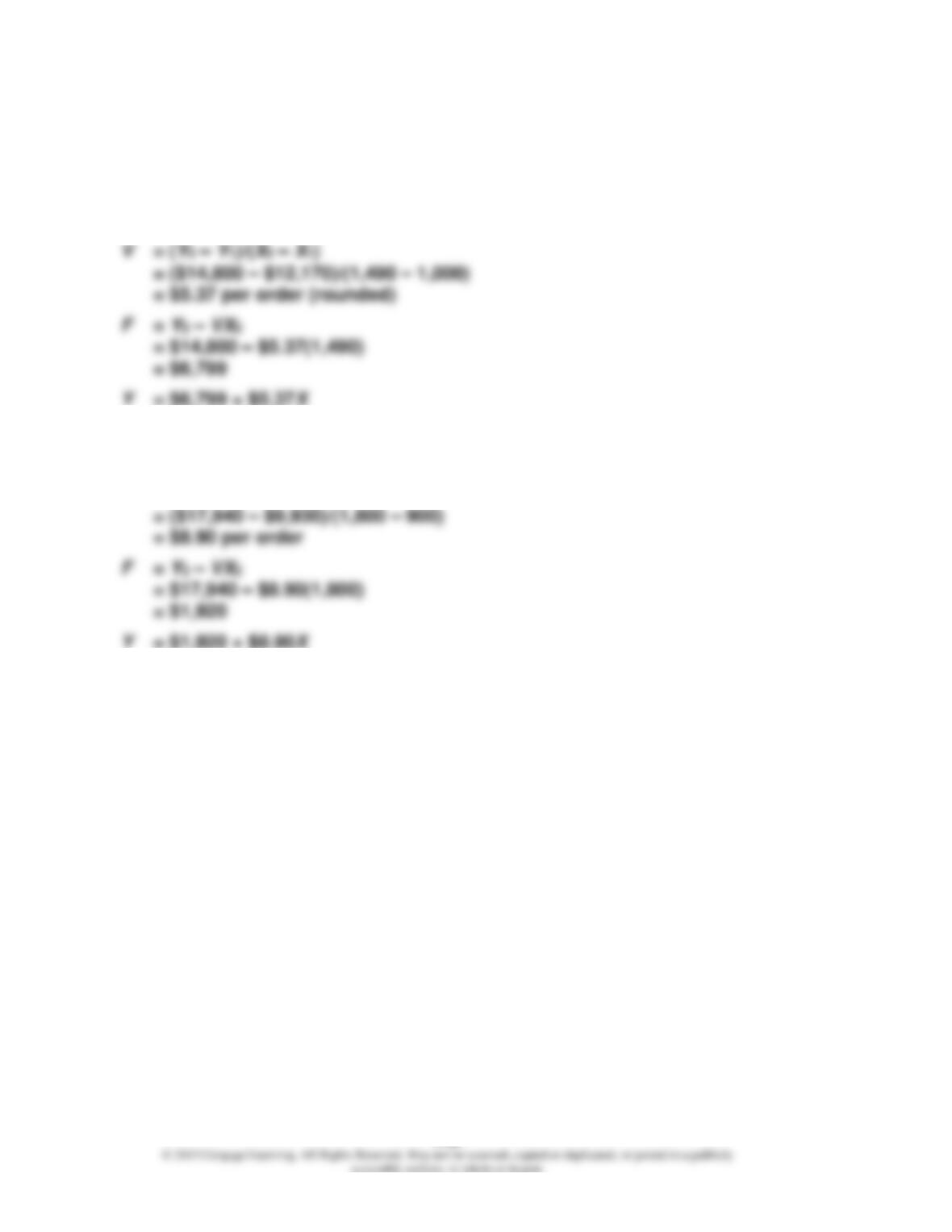
1. Scattergraph:
3-28
Problem 3.33 (Continued)
2. If points 1 and 8 are chosen:
Point 1: 1,000, $12,170
Point 8: 1,490, $14,800
3. High: 1,800, $17,940
Low: 900, $9,930
V = (Y2 – Y1)/(X2 – X1)
3-29
Problem 3.33 (Concluded)
4. Regression output from spreadsheet:
SUMMARY OUTPUT
Regression Statistics
Multiple R
0.905998
R Square
0.820832
Adjusted R Square
ANOVA
df
SS
MS
F
Regression
1
37618885
37618885
36.65077
Residual
8
8211318
1026415
Total
9
45830203
Coefficients
Standard Error
t Stat
P-value
Intercept
2.866748
5. Se = $1,013 (rounded)
Yf = $4,638 + $6.99(1,200)
Problem 3.34
1. The order should cover the variable costs described in the activity cost for-
mulas. These variable costs represent the increase in resource spending—
they are resources acquired as needed.
Material costs ($80 × 20,000) …………………………..… $1,600,000
Labor costs ($20 × 20,000) ………………………………… 400,000
2. The correlation coefficients indicate the reliability of the cost formulas. Of the
four formulas, overhead activity may be a problem. A correlation coefficient
of 0.75 means that only about 56 percent of the variability on overhead cost is
explained by direct labor hours. This can have a bearing on the answer to
3. Resource spending attributable to order:
Materials ($80 × 20,000) ……………………………………. $1,600,000
Labor ($20 × 20,000) …………………………………………. 400,000
Problem 3.35
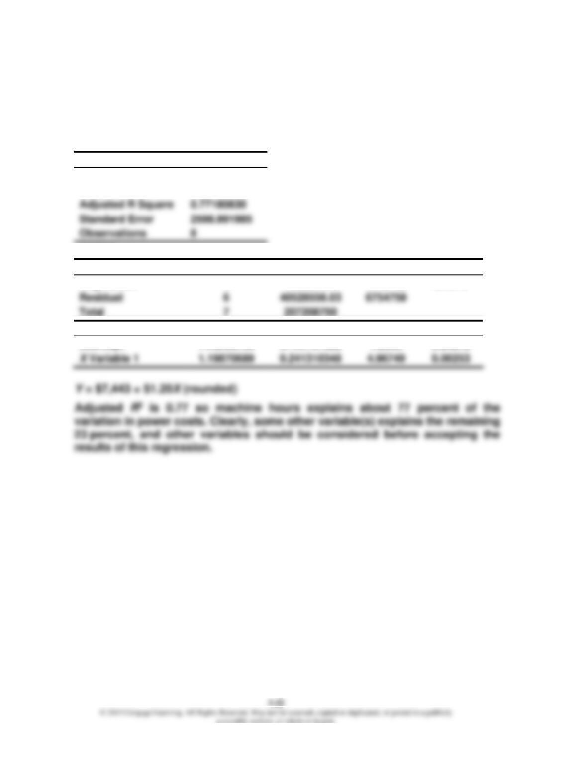
1. Scattergraph:
Scattergraph of Power Activity
$40,000
$50,000
2. High: 30,000, $42,500
Low: 18,000, $31,400
V = (Y2 – Y1)/(X2 – X1)
Problem 3.35 (Continued)
3. Regression output from spreadsheet:
SUMMARY OUTPUT
Regression Statistics
Multiple R
0.89688746
R Square
0.80440712
Adjusted R Square
0.77180830
ANOVA
df
SS
MS
F
Regression
1
166680194
1.7E+08
24.676
Residual
6
Coefficients
Standard Error
t Stat
P-value
Intercept
7442.88793
5744.757622
1.2956
0.24272