
chapter
21
Cost Behavior and Cost-
Volume-Profit Analysis
______________________________________________
OPENING COMMENTS
In Chapter 21, students learn how to conduct cost-volume-profit analysis. In preparation for this activity,
the chapter discusses variable, fixed, and mixed costs.
Cost-volume-profit analysis is conducted using both a formula-based mathematical approach and a
graphic approach. It is applied to single-product and multiple-product companies. The chapter concludes
with an appendix that discusses variable costing.
After studying the chapter, your students should be able to:
1. Classify costs as variable costs, fixed costs, or mixed costs.
2. Compute the contribution margin, the contribution margin ratio, and the unit contribution margin.
3. Determine the break-even point and sales necessary to achieve a target profit.
4. Using a cost-volume-profit chart and a profit-volume chart, determine the break-even point and sales
necessary to achieve a target profit.
5. Compute the break-even point for a company selling more than one product, the operating leverage,
and the margin of safety.
KEY TERMS
absorption costing
activity bases (drivers)
break-even point
contribution margin
contribution margin ratio

390 Chapter 21 Cost Behavior and Cost-Volume-Profit Analysis
cost behavior
cost-volume-profit analysis
cost-volume-profit chart
fixed costs
high-low method
margin of safety
mixed costs
operating leverage
profit-volume chart
relevant range
sales mix
unit contribution margin
variable costing
variable costs
STUDENT FAQS
• Why does variable cost per unit stay the same but total cost varies with the number of units you
produce?
• How do you choose what activity base to use?
• Why does fixed cost remain the same in total dollar amount but increase or decrease per unit as the
level of activity changes?
• What do increases in fixed cost do to break-even analysis?
• What do increases in variable cost do to break-even analysis?
OBJECTIVE 1
Classify costs as variable costs, fixed costs, or mixed costs.
SYNOPSIS
Cost behavior is the manner in which a cost changes as activity changes. Managers find this relationship
useful as it allows managers to predict profits as sales and production volume change. Activity bases are
the things that cause cost to change, and the range over which the changes are of interest is called the
relevant range. Costs are classified as variable, fixed, or mixed costs. Variable costs are those that change
directly in proportion to changes in production volume. Direct materials and direct labor are usually
variable costs. Variable costs have certain characteristics, such as the cost per unit remains the same and
total cost varies in proportion to the activity base. Exhibit 1 shows a graphical representation of variable
cost per unit and variable total cost. Fixed costs are those that remain the same in total over the relevant
range. Straight-line depreciation is an example of a fixed cost. Although total cost remains the same, fixed
cost per unit decreases as production increases. Mixed costs have characteristics of both a variable and
fixed cost. They are also called semivariable or semifixed costs. An example might be a rental car that has
a fixed component (charge per day) and also charges per mile driven. For purposes of analysis, mixed
costs are usually separated into their fixed and variable components. The high-low method is a cost
estimation tool that is used to calculate mixed costs. To calculate, you must have several periods of

Chapter 21 Cost Behavior and Cost-Volume-Profit Analysis 391
historical data, including units produced and total costs. Subtract the lowest levels of production from the
highest levels of production computed as: variable cost per unit = difference in total cost/difference in
units produced. The fixed cost is then estimated by subtracting the total variable costs from the total fixed
costs, as follows: fixed cost = total costs – (variable cost per unit × units produced). Mixed costs contain a
fixed component even if nothing is produced.
Key Terms and Definitions
• Activity Base (Driver) – A measure of activity that is related to changes in cost. Used in
analyzing and classifying cost behavior. Activity bases are also used in the denominator in
calculating the predetermined factory overhead rate to assign overhead costs to cost objects.
• Cost Behavior – The manner in which a cost changes in relation to its activity base (driver).
• Fixed Costs – Costs that tend to remain the same in amount, regardless of variations in the level
of activity.
• High-Low Method – A technique that uses the highest and lowest total costs as a basis for
estimating the variable cost per unit and the fixed cost component of a mixed cost.
• Mixed Costs – Costs with both variable and fixed characteristics, sometimes called semivariable
or semifixed costs.
• Relevant Range – The range of activity over which changes in cost are of interest to
management.
• Variable Costing – The concept that considers the cost of products manufactured to be composed
only of those manufacturing costs that increase or decrease as the volume of production rises or
falls (direct materials, direct labor, and variable factory overhead).
• Variable Costs – Costs that vary in total dollar amount as the level of activity changes.
Relevant Example Exercises and Exhibits
• Example Exercise 21-1 High-Low Method
• Exhibit 1 – Variable Cost Graphs
• Exhibit 2 – Variable Costs and Their Activity Bases
• Exhibit 3 – Fixed Cost Graphs
• Exhibit 4 – Fixed Costs and Their Activity Bases
• Exhibit 5 – Mixed Costs
• Exhibit 6 – Variable and Fixed Cost Behavior
• Exhibit 7 – Variable, Fixed, and Mixed Cost
SUGGESTED APPROACH
Knowing how costs behave enables management to estimate costs when evaluating alternative operating
proposals. Begin your coverage of this objective by reviewing the definitions of variable, fixed, and
mixed costs. Be sure to point out the behavior of both total and unit costs. For example, variable costs are
illustrated in text Exhibit 1. When reviewing this illustration, stress that as the number of units produced
increases, the total direct materials cost increases but the unit cost remains constant.
Fixed costs are shown in text Exhibit 2. This illustration compares the supervisor’s salary in a plant that
makes perfume to the number of perfume bottles produced. The total salary is constant at all production
levels. As a result, the per-unit cost decreases as production increases.
392 Chapter 21 Cost Behavior and Cost-Volume-Profit Analysis
Mixed costs have both a fixed and a variable component. An example of a mixed cost is the price paid to
rent a moving van if that price includes a fixed fee plus a charge per mile (i.e., $50 plus $0.30 per mile).
In addition to understanding how costs behave, managers need to know what activities create costs. These
activities are called activity bases (or activity drivers). Ask your students to identify the activity base that
drives their textbook expenditures. (Answer: the number of courses taken)
GROUP LEARNING ACTIVITY—Variable, Fixed, and Mixed Costs
Divide your class into small groups. Ask them to list examples of fixed, variable, and mixed costs
incurred by a McDonald’s restaurant. Encourage them to list as many examples as they can. Also instruct
them to identify the activity base (driver) for each variable cost on their list.
Possible response: McDonald’s variable costs could include all the food and drinks, hourly labor, food
containers, and condiments. Fixed costs could include rent or mortgage, managers’ salaries, insurance,
and franchise fees. Mixed costs could include utilities, advertising, and maintenance costs.
DEMONSTRATION PROBLEM—High-Low Method
For most business analysis, mixed costs must be separated into their fixed and variable components. Use
the following problem to demonstrate the high-low method.
The power costs of Jones Manufacturing behave as a mixed cost. The activity that creates most of the
power costs is machine usage. Therefore, power costs will be analyzed in relation to machine hours.
Machine hours and power costs for the past six months are presented on Transparency Master (TM) 21-1.
Ask students to identify the highest and lowest levels of power usage (August and July respectively).
Next, ask them to compute the difference in machine hours and power costs and record these numbers in
their notes.
Once the high and low points have been identified, the variable portion of the cost is determined using the
following equation:
Difference in Total Cost
Variable Cost/Unit Difference in Machine Hours
$300
Variable Cost/Unit $0.05/hour
6,000 hours
=
==
The fixed portion can be determined using data from either the high or the low power-usage points and
the following equation:
Total Cost = (Variable Cost/Unit No. of Units) + Fixed Costs
Chapter 21 Cost Behavior and Cost-Volume-Profit Analysis 393
Using data from July:
$1,900 = ($0.05/unit 14,000) + Fixed Costs
$1,900 – $700 = Fixed Costs
$1,200 = Fixed Costs
OBJECTIVE 2
Compute the contribution margin, the contribution margin ratio, and the unit contribution
margin.
SYNOPSIS
Cost-volume-profit analysis is useful for managerial decision making. The analysis may be used to
analyze the following: the effects of changes in selling price on profits, the effects of changes in costs of
profits, the effects of changes in volume on profits, how to set prices, how to select the mix of products to
sell, and how to choose marketing strategy. The contribution margin provides insights in to the profit
potential and is calculated as: contribution margin = sales – variable costs. The contribution margin can
also be expressed as a percentage; this ratio is calculated as: contribution margin ratio = contribution
margin/sales. This ratio is most useful when the increase or decrease in sales volume is measured in sales
dollars. The contribution margin can also be computed per unit as: unit contribution margin = sales price
per unit – variable cost per unit.
Key Terms and Definitions
• Contribution Margin – Sales less variable costs and variable selling and administrative
expenses.
• Contribution Margin Ratio – The percentage of each sales dollar that is available to cover the
fixed costs and provide an operating income.
• Cost-Volume-Profit Analysis – The systematic examination of the relationships among selling
prices, volume of sales and production, costs, expenses, and profits.
• Unit Contribution Margin – The dollars available from each unit of sales to cover fixed costs
and provide operating profits.
Relevant Example Exercises and Exhibits
• Example Exercise 21-2 Contribution Margin
• Exhibit 8 – Contribution Margin Income Statement Format
SUGGESTED APPROACH
Give students the following formulas related to contribution margin (CM):
CM = Sales – Variable Costs
CM Ratio = CM/Sales

394 Chapter 21 Cost Behavior and Cost-Volume-Profit Analysis
Stress that contribution margin is the amount of funds left from a sale after the variable costs have been
paid. Contribution margin is used to pay the fixed costs of the business. Once all fixed costs have been
covered, any contribution margin left represents profit.
The contribution margin ratio tells what percent of each sales dollar is contribution margin. Once again, if
sales are above break-even, this percentage represents profit.
GROUP LEARNING ACTIVITY—Contribution Margin
Give your students the following sales and cost data for Van Buren Company. The total sales and cost
information is based on the sale of 20,000 units.
Total Per Unit
Sales $570,000 $28.50
Variable costs $387,600 $19.38
Fixed costs $140,000
Divide the class into small groups. Ask students to compute the total contribution margin, contribution
margin ratio, and unit contribution margin for this company. Also instruct them to compute the increase
in net income that will result from a $50,000 increase in sales and a 1,000-unit increase in sales.
The answers to this exercise are as follows:
1. Total contribution margin: $182,400
2. Contribution margin ratio: 32 percent
3. Unit contribution margin: $9.12
4. Increase in net income from $50,000 increase in sales: $50,000 32% = $16,000
5. Increase in net income from 1,000-unit increase in sales: 1,000 $9.12 = $9,120
OBJECTIVE 3
Determine the break-even point and sales necessary to achieve a target profit.
SYNOPSIS
The cost-volume-profit analysis allows a business to determine the break-even point in sales and to
determine the sales needed to make a desired profit. The break-even point is the level of sales at which a
company’s revenues and expenses are equal. It is computed as follows: break-even sales units = fixed
costs/unit contribution margin. This number can also be computed using sales dollars as follows: break-
even sales (dollars) = fixed costs/contribution margin ratio. The break-even point is affected by changes
in fixed costs, unit variable costs, and the unit selling price. Unit variable costs do not change with level
of activity; however, unit variable costs may be affected by changes in the price of materials, labor, or
sales. An increase in unit variable costs increases the break-even point, and decreases in variable costs
decrease the break-even point. If the selling price changes, this also changes the break-even point in the

Chapter 21 Cost Behavior and Cost-Volume-Profit Analysis 395
opposite direction. If the sales price increases, the break-even point decreases, and if the sales price
decreases, the break-even point increases. A summary of the effects is shown in Exhibit 13. By modifying
the break-even equation, a business can determine what sales are necessary to achieve a target profit. The
equation is: sales (units) = (fixed costs + target profit)/unit contribution margin.
Key Terms and Definitions
• Break-Even Point – The level of business operations at which revenues and expired costs are
equal.
Relevant Example Exercises and Exhibits
• Example Exercise 21-3 Break-Even Point
• Example Exercise 21-4 Target Profit
• Exhibit 9 – Break-Even Point
• Exhibit 10 – Effect of Change in Fixed Costs on Break-Even Point
• Exhibit 11 – Effect of Change in Unit Variable Cost on Break-Even Point
• Exhibit 12 – Effect of Change in Unit Selling Price on Break-Even Point
• Exhibit 13 – Effects of Changes in Selling Price and Costs on Break-Even Point
SUGGESTED APPROACH
Under this objective, the text presents formulas to calculate the break–even point in units and the unit
sales necessary to achieve a target profit. Use the following lecture notes to explain these formulas.
LECTURE NOTES—Break–Even Point and Target Profit
Although students generally like to use a “formula” in solving accounting problems, they dislike
memorizing them. Remind students that they can use the following formula to solve both break-even and
target profit problems as long as they remember that profit is zero at the break-even point.
Fixed Costs + Target Profit
Sales (units) Unit Contribution Margin
=
Many students benefit from seeing formulas derived from equations they already understand. The text’s
formula can be derived as follows:
Sales Price (X) – Variable Cost (X) – Fixed Costs = Income from Operations
where: X = No. of units sold
also note: sales price and variable cost are per-unit amounts

396 Chapter 21 Cost Behavior and Cost-Volume-Profit Analysis
. . . or (solving for X)
Sales Price (X) – Variable Cost (X) = Fixed Costs + Income from Operations
X (Sales Price – Variable Cost) = Fixed Costs + Income from Operations
X = (Fixed Costs + Income from Operations)/(Sales Price – Variable Cost)
X = (Fixed Costs + Income from Operations)/Unit Contribution Margin
Note: “Target profit” is a company’s desired income from operations.
In reality, students also can solve break-even and target profit problems using the equation:
Sales Price (X) – Variable Cost (X) – Fixed Costs = Income from Operations. Some of your students will
find this equation easiest to remember and use.
GROUP LEARNING ACTIVITY—Break-Even and Target Profit
One of the true benefits of cost-volume-profit analysis is that a business can analyze a variety of “what-if”
scenarios. TM 21-2 presents several what-ifs for your students to answer in small groups. Solutions are
presented on TM 21-3.
WRITING EXERCISE—Break-Even Point
Ask your students to write an answer to the following questions (TM 21-4):
Would an increase in variable costs per unit cause a company’s break-even point to
increase or decrease? Why?
Possible response: An increase in variable costs will cause the break-even point in unit
sales to increase. An increase in variable costs leaves less contribution margin to apply
toward fixed costs, requiring more units to be sold to cover the fixed costs.
Would an increase in per-unit selling price cause a company’s break-even point to
increase or decrease? Why?
Possible response: An increase in sales price will cause the break-even point in unit sales
to decrease. An increased sales price provides additional contribution margin to cover
fixed costs, requiring fewer sales to break even.
OBJECTIVE 4
Using a cost-volume-profit chart and a profit-volume chart, determine the break-even point
and sales necessary to achieve a target profit.
SYNOPSIS
Managers often want to know a business’s profit at multiple sales, costs, and the related profits. To
achieve this, a cost-volume-profit chart is constructed over the relevant range. The horizontal axis of the

Chapter 21 Cost Behavior and Cost-Volume-Profit Analysis 397
chart is the sales volume expressed in units; the vertical axis displays the dollar amounts of total sales and
total costs. A total sales line is plotted by connecting the point at zero on the left corner of the graph to a
second point on the chart. A total cost line is plotted by beginning with total fixed costs on the vertical
axis. A second point is determined by multiplying the maximum number of units in the relevant range,
which is found on the far right of the horizontal axis by the unit variable costs and adding the total fixed
costs. Another useful chart is the profit-volume chart; it plots only the difference between total sales and
total costs. This chart allows managers to determine the operating profit (or loss) for various levels of
units sold. This graphic approach is made easier by computers. Managers can vary assumptions regarding
selling process, costs, and volume and observe the effects of each change on the break-even point and
profit. An analysis like this is called a “what if” or sensitivity analysis. This graphical analysis depends on
assumptions as follows: total sales and total costs can be represented by straight lines, costs can be
divided into fixed and variable costs, sales mix is constant, there is no change in inventory quantities, and
the number is within the relevant range.
Key Terms and Definitions
• Cost-Volume-Profit Chart – A chart used to assist management in understanding the
relationships among costs, expenses, sales, and operating profit or loss.
• Profit-Volume Chart – A chart used to assist management in understanding the relationship
between profit and volume.
Relevant Example Exercises and Exhibits
• Exhibit 14 – Cost-Volume-Profit Chart
• Exhibit 15 – Revised Cost-Volume-Profit Chart
• Exhibit 16 – Profit-Volume Chart
• Exhibit 17 – Original Profit-Volume Chart and Revised Profit-Volume Chart
SUGGESTED APPROACH
The mathematical (formula-based) approach to calculating a break-even point is usually more accurate
than the graphic approach. Most students also find the mathematical approach to be a quicker and easier
way to solve problems. However, because it is important that students learn how to read business graphs,
the graphic approach to break-even analysis deserves attention.
Use Exhibit 5 in the text to review the construction of a cost-volume-profit (CVP) chart. Emphasize that a
CVP chart provides a visual representation of the break-even point. The chart consists of a sales line and a
cost line. The intersection of these lines is the break-even point.
Exhibit 7 illustrates a profit-volume (PV) chart. A profit line is plotted on a PV chart. The break-even
point occurs where the profit line intersects the zero horizontal profit line. This represents the point where
profits equal zero.
You may want to focus on the interpretation rather than the preparation of break-even graphs. The group
learning activity that follows will ask students to read and interpret cost-volume-profit (CVP) and profit-
volume (PV) charts.

398 Chapter 21 Cost Behavior and Cost-Volume-Profit Analysis
GROUP LEARNING ACTIVITY—CVP and PV Charts
Handout 21-1 presents a CVP chart and a PV chart. It also poses several questions to test your students’
ability to read and interpret these graphs. Distribute copies of the handout to your students and ask them
to work in small groups to answer the questions.
Handout 21-1 solutions:
Chart 1: Question—See Exhibit 5 in the text for sales and cost line identification; Question 2—40,000
units; Question 3—$40,000; Question 4—Variable cost $.50 per unit [VC = ($60,000 – $40,000)/40,000)];
Question 5—profit at 80,000 units is $40,000 [CM × (Unit Sales – Break-Even Units)] OR [($1 × (80,000
– 40,000)]
Chart 2: Question 1—15,000 units; Question 2—$25,000; Question 3—$25,000 [CM × (Unit Sales –
Break-Even Units)] OR [1.67 × (30,000 – 15,000)]
OBJECTIVE 5
Compute the break-even point for a company selling more than one product, the operating
leverage, and the margin of safety.
SYNOPSIS
The sales mix is the relative distribution of sales among the products sold by a company. For break-even
analysis, it is useful to think of the unit selling price as a constant. The constant is the sum of the unit
selling prices of each product multiplied by the sale mix percentage. The equation using E as the constant
is: break-even sales (units) for E = fixed costs/unit contribution margin. If the sales mix changes, the
break-even point for E can be recomputed. The relationship between a company’s contribution margin
and income from operations is measured by operating leverage, computed as: operating leverage =
contribution margin/income from operations. The difference between contribution margin and income
from operations is fixed costs. The impact of a change in sales on income from operations for companies
with high and low operating leverage is summarized in Exhibit 20. The margin of safety indicates the
possible decrease in sales that may occur before an operating loss results. It may be expressed as dollars
of sales, units of sales, or a percent of current sales. The equation is: margin of safety = (sales – sales at
break-even point/sales.
Key Terms and Definitions
• Margin of Safety – Indicates the possible decrease in sales that may occur before an operating
loss results.
• Operating Leverage – A measure of the relative mix of a business’s variable costs and fixed
costs, computed as contribution margin divided by operating income.
• Sales Mix – The relative distribution of sales among the various products available for sale.
Relevant Example Exercises and Exhibits
• Example Exercise 21-5 Sales Mix and Break-Even Analysis
Chapter 21 Cost Behavior and Cost-Volume-Profit Analysis 399
• Example Exercise 21-6 Operating Leverage
• Example Exercise 21-7 Margin of Safety
• Exhibit 18 – Multiple Product Sales Mix
• Exhibit 19 – Break-Even Sales: Multiple Products
• Exhibit 20 – Effect of Operating Leverage on Income from Operations
SUGGESTED APPROACH
Cost-volume-profit analysis can be applied to companies that sell more than one product, as long as their
sales mix is constant. Use the Demonstration Problem to illustrate this modification to basic break-even
analysis.
Ask your students to identify examples of sales mixes for various real-life businesses. An example would
be car dealerships that sell different makes of cars, such as Cadillacs and Buicks.
DEMONSTRATION PROBLEM—Sales Mix
To calculate the break-even point for a company that sells more than one product, a weighted average
contribution margin must be determined. The text illustrates this calculation by multiplying the sales price
and then the unit variable cost by the sales mix percentage and adding these two amounts. The calculation
can also be performed directly on the unit contribution margin.
For example, assume that a gourmet food manufacturer has considered renting a booth at a local mall to
sell gift boxes of candy, nuts, and cookies during the holiday season. The fixed costs to rent and operate
the booth would be $27,900. The unit contribution margins and sales mix anticipated by the company are
as follows:
Unit Contribution Margin Sales Mix
Candy $1.50 50%
Nuts $2.00 30%
Cookies $1.00 20%
A weighted average unit contribution margin would be as follows:
$1.50 50% = $0.75
$2.00 30% = 0.60
$1.00 20% = 0.20
$1.55
To break even, the company would need to sell 18,000 gift boxes ($27,900/$1.55). Using the sales mix,
the number of each type of gift box can be calculated.
Candy: 18,000 50% = 9,000
Nuts: 18,000 30% = 5,400
Cookies: 18,000 20% = 3,600
18,000

400 Chapter 21 Cost Behavior and Cost-Volume-Profit Analysis
DEMONSTRATION PROBLEM—Operating Leverage
Operating leverage compares contribution margin to operating income. The formula is:
Contribution Margin
Operating Leverage Operating Income
=
Ask your students to calculate the operating leverage of a company with $800,000 in sales, $200,000 in
variable costs, and $400,000 in fixed costs.
Operating Leverage = $600,000/$200,000 = 3
An operating leverage of 3 indicates that operating income will increase three times any percentage
increase in sales. For example, if sales increase 5 percent, operating income will increase 15 percent. You
may want to prove this by presenting the follow example.
Original Data + 5% in Sales
Sales $800,000 $840,000
Variable costs 200,000 210,000
Contribution margin $600,000 $630,000
Fixed costs 400,000 400,000
Operating income $200,000 $230,000
$30,000
15% increase
$200,000 =
Stress that large amounts of fixed costs cause companies in capital-intensive industries to have a high
operating leverage. Operating leverage is much lower in labor-intensive industries.
GROUP LEARNING ACTIVITY—Margin of Safety
Explain that margin of safety measures the amount by which current sales exceed sales at the break-even
point. It may be expressed in dollars, in units, or as a percentage. When expressed as a percentage, margin
of safety shows the percentage that sales can drop without resulting in an operating loss. The formula to
calculate margin of safety as a percentage of current sales is as follows:
Sales Sales at Break–Even Point
Margin of Safety Sales
−
=
Ask your students to work in small groups to answer questions related to margin of safety on TM 21-5.
The solutions are provided on TM 21-6.

Chapter 21 Cost Behavior and Cost-Volume-Profit Analysis 401
INTERNET ACTIVITY—Review of Chapter Concepts
CCH Business Owner’s Toolkit is an excellent Web site for reviewing cost-volume-profit analysis and
related topics from the chapter. Direct your students to the following Web site:
http://www.toolkit.cch.com/text/P06_7500.asp
This Web site will present information on using cost-volume-profit analysis in a small business. It also
has links to information on breakeven analysis, contribution margin analysis, and operating leverage. The
breakeven analysis page includes an interactive calculator that will compute breakeven points and
produce a cost-volume-profit graph.
APPENDIX—VARIABLE COSTING
SYNOPSIS
GAAP accounting requires absorption costing for financial statements. The previous chapters have shown
absorption costing. Alternative reports may be prepared using variable or direct costing. These are for use
in internal decision making. In variable costing, fixed factory overhead costs do not become a part of the
cost of goods manufactured. Fixed factory overhead costs are treated as a period expense. Exhibit 21
illustrates the differences between absorption and variable costing in the cost of goods manufactured.
Absorption costing is often used by managers to avoid misinterpretations of changes of inventory levels
as increases or decreases in income. Variable costing is used by managers for cost control, product
pricing, and production planning.
Key Terms and Definitions
• Absorption Costing – The reporting of the costs of manufactured products, normally direct
materials, direct labor, and factory overhead, as product costs.
Relevant Example Exercises and Exhibits
• Exhibit 21 – Absorption Versus Variable Cost of Goods Manufactured
• Exhibit 22 – Variable Costing Income Statement
• Exhibit 23 – Absorption Costing Income Statement
• Exhibit 24 – Relationship Between Variable and Absorption Costing Income
• Exhibit 25 – Units Manufactured Exceed Units Sold
SUGGESTED APPROACH
Explain that the name given to the manufacturing cost system your students have been learning is
absorption costing. Under absorption costing, all costs necessary to manufacture a product are “absorbed”
by the product (included in the product’s reported cost). This includes both fixed and variable
manufacturing costs. Review absorption costing with the group learning activity that follows.

402 Chapter 21 Cost Behavior and Cost-Volume-Profit Analysis
Explain that variable costing is another approach used for management reporting. Under variable costing,
only variable costs are included in the product costs reported as cost of goods sold or ending inventory.
All fixed costs are treated as period expenses. The group learning activity and the lecture aids that follow
will help you present the basics of variable costing.
GROUP LEARNING ACTIVITY—Absorption and Variable Costing
To review absorption costing, ask your students to prepare an income statement for Laurens Incorporated,
using the data on TM 21-7.
TM 21-8 displays Laurens’ income statement under absorption costing. It also shows the company’s
income statement under variable costing. Point out the $30,000 difference in the two income statements.
Ask students to examine the income statements, silently on their own, and look for the reason the
statements present a different net income. After a minute, ask them to share their ideas in their group.
This group discussion time will allow students to finalize their answers before sharing them with the
class.
Through discussion, bring the class to a consensus that the $30,000 difference is the fixed cost of the
2,000 units produced but not sold ($15/unit 2,000 units). Under full absorption costing, this $30,000
cost is allocated to the units in the ending finished goods inventory. Therefore, it is carried on the balance
sheet as an asset. Under variable costing, this $30,000 is reported on the income statement as a period
expense. As a result, net income is $30,000 lower under variable costing.
LECTURE AID—Variable Costing
Although variable costing is not permitted for financial reporting, many managers find it useful for
management reporting. Variable costing tends to show costs in the same manner as they are incurred:
variable costs on a per-unit basis and fixed costs in total.
Another benefit of variable costing is the ability to isolate the impact of changes in sales or costs. TM 21-
9 shows an income statement for Laurens Incorporated, assuming sales of 20,000 units and 30,000 units.
Point out that as volume increases, only variable costs change. This is clearly evident from the variable
costing income statement.
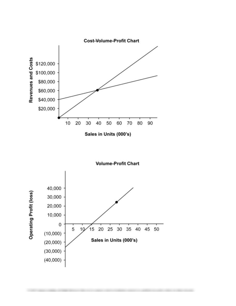
Handout 21-1
1. Identify the sales
and cost lines.
2. What is the break-
even point in units?
3. What is the
company’s total
fixed cost?
4. What is the
company’s variable
cost per unit?
5. What is the
company’s profit at
sales of 80,000
units?
1. What is this
company’s break–
even point in units?
2. What is the company’s
total fixed cost?
3. What is the company’s
profit at sales of
30,000 units?
Type Item Description LO(s) Difficulty Time Est BUSPROG AICPA ACBSP – APC Bloom’s EE Excel GL SMH FAI Service Real World Writing Ethics Internet Group
DQ 1 1 Easy 5 min. Analytic Measurement Variable and Fixed Costs Remembering
DQ 2 1 Easy 5 min. Analytic Measurement Variable and Fixed Costs Remembering
DQ 3 1 Easy 5 min. Analytic Measurement Variable and Fixed Costs Remembering
DQ 4 1 Easy 5 min. Analytic Measurement Variable and Fixed Costs Remembering
DQ 5 2 Easy 5 min. Analytic Measurement Variable and Fixed Costs Remembering
DQ 6 2 Easy 5 min. Analytic Measurement Contribution Margin Remembering
DQ 7 3 Easy 5 min. Analytic Measurement Break-even point Remembering
DQ 8 3 Easy 5 min. Analytic Measurement Break-even point Remembering
DQ 9 5 Easy 5 min. Analytic Measurement Break-even point Remembering
DQ 10 5 Easy 5 min. Analytic Measurement Break-even point Remembering
PE 1A High-low method 1 Easy 10 min. Analytic Measurement Variable and Fixed Costs Applying x
PE 1B High-low method 1 Easy 10 min. Analytic Measurement Variable and Fixed Costs Applying x
PE 2A Contribution margin 2 Easy 10 min. Analytic Measurement Contribution Margin Applying x
PE 2B Contribution margin 2 Easy 10 min. Analytic Measurement Contribution Margin Applying x
PE 3A Break-even point 3 Easy 10 min. Analytic Measurement Break-even point Applying x
PE 3B Break-even point 3 Easy 10 min. Analytic Measurement Break-even point Applying x
PE 4A Target profit 3 Easy 10 min. Analytic Measurement Margin of safety/sales target Applying x
PE 4B Target profit 3 Easy 10 min. Analytic Measurement Margin of safety/sales target Applying x
PE 5A Sales mix and break-even analysis 5 Easy 10 min. Analytic Measurement Margin of safety/sales target Applying x
PE 5B Sales mix and break-even analysis 5 Easy 10 min. Analytic Measurement Margin of safety/sales target Applying x
PE 6A Operating leverage 5 Easy 5 min. Analytic Measurement CVP Analysis Applying x
PE 6B Operating leverage 5 Easy 5 min. Analytic Measurement CVP Analysis Applying x
PE 7A Margin of safety 5 Easy 5 min. Analytic Measurement Margin of safety/sales target Applying x
PE 7B Margin of safety 5 Easy 5 min. Analytic Measurement Margin of safety/sales target Applying x
EX 1 Classify costs 1 Easy 15 min. Analytic Measurement Variable and Fixed Costs Remembering
EX 2 Identify cost graphs 1 Easy 15 min. Analytic Measurement CVP Analysis Applying
EX 3 Identify activity bases 1 Easy 15 min. Analytic Measurement Managerial Accounting Features/Costs Remembering
EX 4 Identify activity bases 1 Easy 15 min. Analytic Measurement Managerial Accounting Features/Costs Remembering
EX 5 Identify fixed and variable costs 1 Easy 15 min. Analytic Measurement Variable and Fixed Costs Remembering
EX 6 Relevant range and fixed and variable costs 1 Moderate 20 min. Analytic Measurement Variable and Fixed Costs Applying x
EX 7 High-low method 1 Easy 15 min. Analytic Measurement Variable and Fixed Costs Applying x x
EX 8 High-low method for service company 1 Moderate 20 min. Analytic Measurement Variable and Fixed Costs Applying x
EX 9 Contribution margin ratio 2 Easy 10 min. Analytic Measurement Contribution Margin Applying x
EX 10 Contribution margin and contribution margin ratio 2 Moderate 15 min. Analytic Measurement Break-even point Applying x
EX 11 Break-even sales and sales to realize income from operations 3 Easy 10 min. Analytic Measurement Break-even point Applying x
EX 12 Break-even sales 3 Moderate 15 min. Analytic Measurement Break-even point Applying
EX 13 Break-even sales 3 Easy 10 min. Analytic Measurement Break-even point Applying x
EX 14 Break-even analysis 3 Easy 10 min. Analytic Measurement Break-even point Applying
EX 15 Break-even analysis 3 Moderate 15 min. Analytic Measurement Break-even point Applying
EX 16 Break-even analysis 3 Moderate 15 min. Analytic Measurement Break-even point Applying x
EX 17 Cost-volume-profit chart 4 Moderate 20 min. Analytic Measurement CVP Analysis Applying x
EX 18 Profit-volume chart 4 Moderate 20 min. Analytic Measurement CVP Analysis Applying
EX 19 Break-even chart 4 Moderate 15 min. Analytic Measurement Break-even point Applying
EX 20 Break-even chart 4 Moderate 15 min. Analytic Measurement Break-even point Applying
EX 21 Sales mix and break-even sales 5 Moderate 15 min. Analytic Measurement Break-even point Applying x
EX 22 Break-even sales and sales mix for a service company 5 Moderate 20 min. Analytic Measurement Break-even point Applying
EX 23 Margin of safety 5 Moderate 15 min. Analytic Measurement Margin of safety/sales target Applying x
EX 24 Break-even and margin of safety relationships 5 Moderate 10 min. Analytic Measurement Margin of safety/sales target Applying x
EX 25 Operating leverage 5 Moderate 15 min. Analytic Measurement CVP Analysis Applying x
EX 26 Items on variable costing income statement Appendix Easy 5 min. Analytic Measurement CVP Analysis Applying
EX 27 Variable costing income statement Appendix Moderate 15 min. Analytic Measurement CVP Analysis Applying x
EX 28 Absorption costing income statement Appendix Moderate 20 min. Analytic Measurement CVP Analysis Applying x
PR 1A Classify costs 1 Moderate 45 min. Analytic Measurement Variable and Fixed Costs Applying
PR 2A Break-even sales under present and proposed conditions 2,3 Challenging 2 hours Analytic Measurement Break-even point Applying x x
PR 3A Break-even sales and cost-volume-profit chart 3,4 Moderate 1 hour Analytic Measurement Break-even point Applying
PR 4A Break-even sales and cost-volume-profit chart 3,4 Challenging 1.5 hours Analytic Measurement Break-even point Applying
PR 5A Sales mix and break-even sales 5 Easy 1.5 hours Analytic Measurement Break-even point Applying x
PR 6A Contribution margin, break-even sales, cost-volume-profit chart, margin of safety, and operating leverage 2,3,4,5 Challenging 1.5 hours Analytic Measurement Contribution Margin Applying x
PR 1B Classify costs 1 Moderate 45 min. Analytic Measurement Variable and Fixed Costs Applying
PR 2B Break-even sales under present and proposed conditions 2,3 Challenging 2 hours Analytic Measurement Break-even point Applying x x
PR 3B Break-even sales and cost-volume-profit chart 3,4 Moderate 1 hour Analytic Measurement Break-even point Applying
PR 4B Break-even sales and cost-volume-profit chart 3,4 Challenging 1.5 hours Analytic Measurement Break-even point Applying
PR 5B Sales mix and break-even sales 5 Easy 1.5 hours Analytic Measurement Break-even point Applying x
PR 6B Contribution margin, break-even sales, cost-volume-profit chart, margin of safety, and operating leverage 2,3,4,5 Challenging 1.5 hours Analytic Measurement Contribution Margin Applying x
CP 1 Ethics and professional conduct business 3 Moderate 15 min. Ethics Measurement Break-even point Analyzing x x
CP 2 Break-even sales, contribution margin 2,3 Moderate 15 min. Analytic Measurement Break-even point Understanding x
CP 3 Break-even analysis 3 Moderate 15 min. Analytic Measurement Break-even point Analyzing x
CP 4 Variable costs and activity bases in decision making 3,4 Moderate 30 min. Analytic Measurement Variable and Fixed Costs Analyzing
CP 5 Variable costs and activity bases in decision making 3,4 Challenging 30 min. Analytic Measurement Variable and Fixed Costs Analyzing x
CP 6 Break-even analysis 3 Moderate 1 hour Analytic Measurement Break-even point Applying
HOMEWORK CHART WITH LEARNING OUTCOMES TAGGING
TAGGING
RESOURCES
FOCUS