20–16
Problem 20.23 (Concluded)
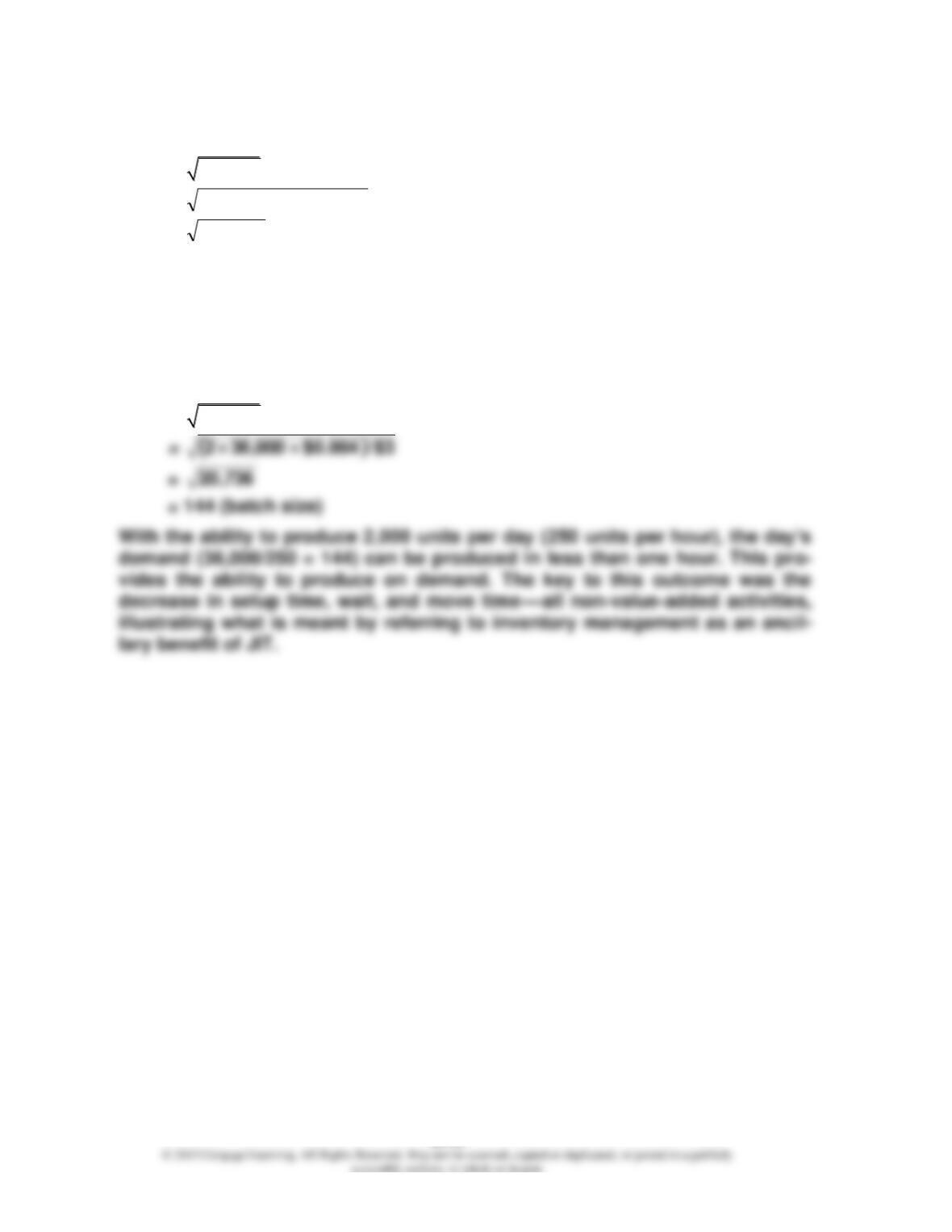
4. EOQ =
2DP / C
=
( )
3$/10$000,362
=
000,240
= 490 (batch size, rounded)
This further reduction in setup time and cost reduces the batch size even
more. As the setup time is reduced to even lower levels and the cost is re-
duced, the batch size becomes even smaller.
If the cost is $0.864, then the batch size is 144:
EOQ =
2DP / C
20–17
Problem 20.24
1. Let X = Model 12 and Y = Model 15
Max Z = $60X + $30Y
subject to:
3X + 0.75Y< 60,000 (1)
X < 15,000 (2)
(Units are in thousands.)
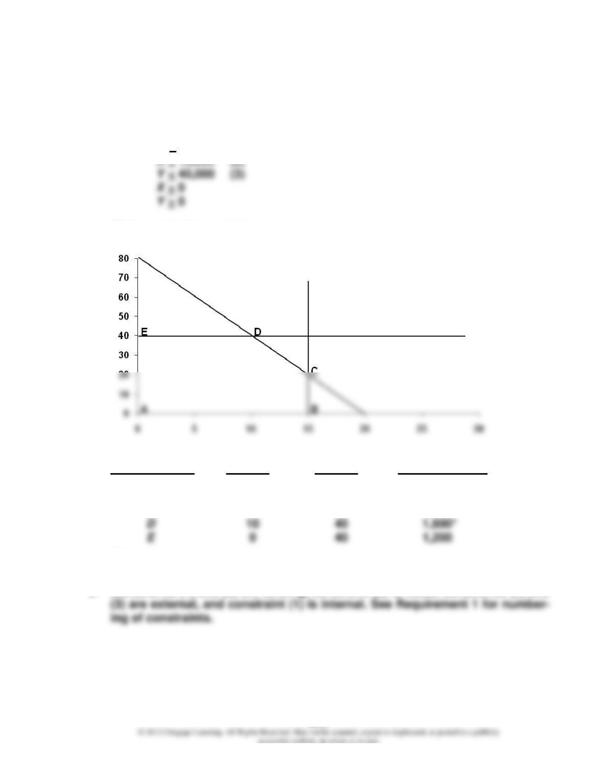
2. Corner Point X-Value Y-Value Z = $60X + $30Y
A 0 0 $ 0
B 15 0 900
C 15 20 1,500
*Optimal solution.
3. Constraints (1) and (3) are binding, constraint (2) is loose, constraints (2) and
20–18
Problem 20.25
1. ($30 × 1,000) + ($60 × 2,000) = $150,000
2. Pocolimpio: CM/qt. = $30/2 = $15/qt. (Two quarts are used for each unit.)
Total contribution margin possible = $15 × 6,000 = $90,000 [involves selling
3. Let X = Number of Pocolimpio produced
Let Y = Number of Maslimpio produced
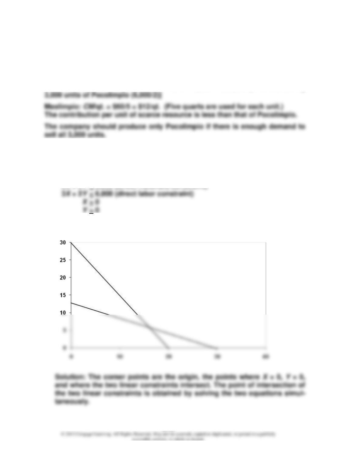
a. Max Z = $30X + $60Y (objective function)
2X + 5Y < 6,000 (direct materials constraint)
b. (Units are in hundreds.)
Problem 20.25 (Concluded)
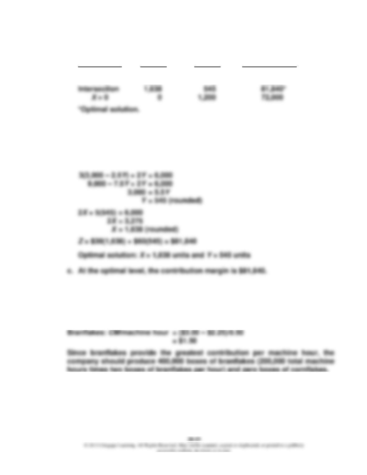
Corner Point X-Value Y-Value Z = $30X + $60Y
Origin 0 0 $ 0
Y = 0 2,000 0 60,000
The intersection values for X and Y can be found by solving the simulta-
neous equations:
2X + 5Y = 6,000
2X = 6,000 – 5Y
X = 3,000 – 2.5Y
Problem 20–26
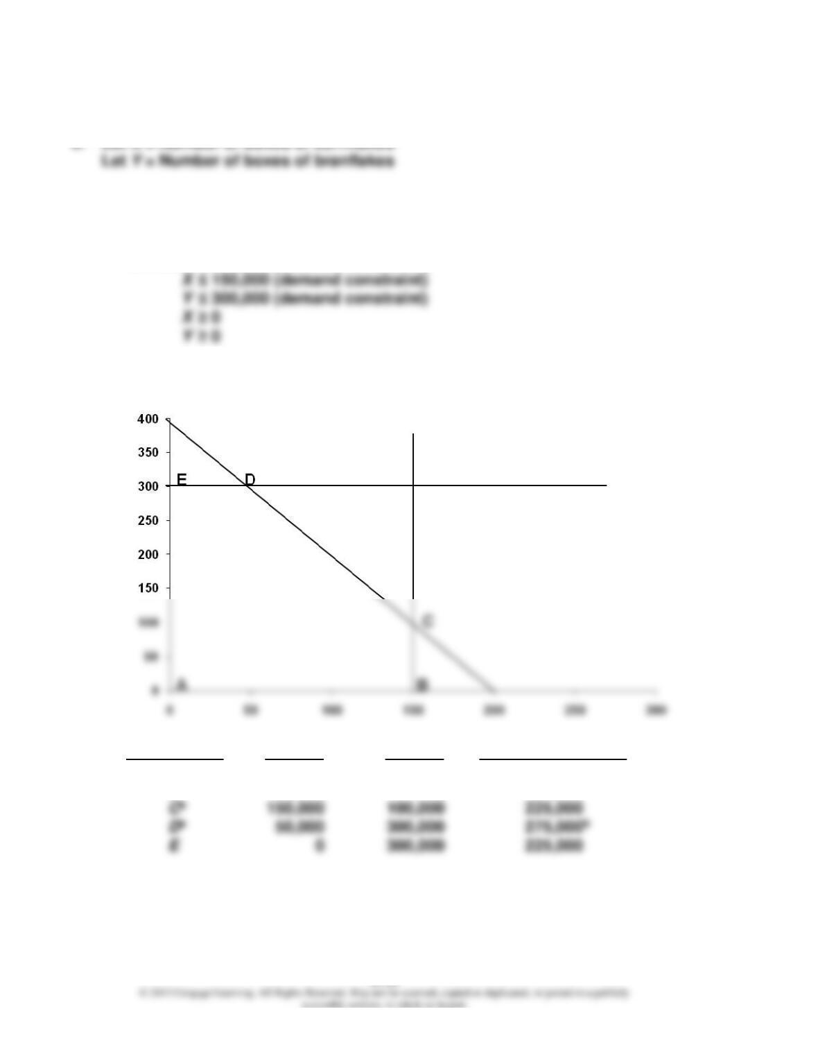
1. Cornflakes: CM/machine hour = ($2.50 – $1.50)/1
= $1.00
20–20
Problem 20.26 (Continued)
a. Formulation:
Z = $1.00X + $0.75Y (objective function)
subject to:
X + 0.5Y ≤ 200,000 (machine constraint)
b. and c. (Units are in thousands.)
Corner Point X-Value Y-Value Z = $1.00X + $0.75Y
A 0 0 $ 0
B 150,000 0 150,000
20–21
Problem 20.26 (Concluded)
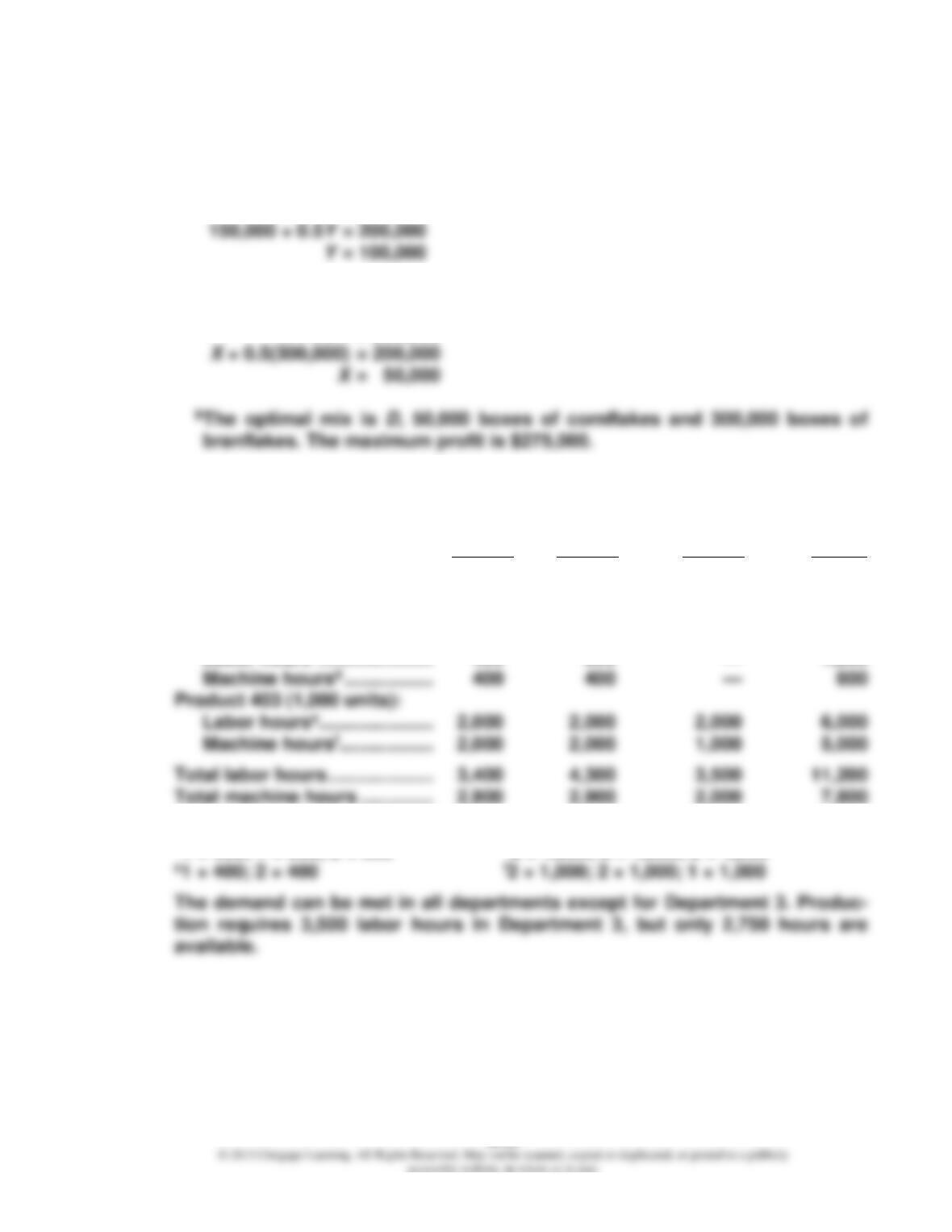
aPoint C:
X = 150,000
X + 0.5Y = 200,000
Point D:
Y = 300,000
X + 0.5Y = 200,000
Problem 20.27
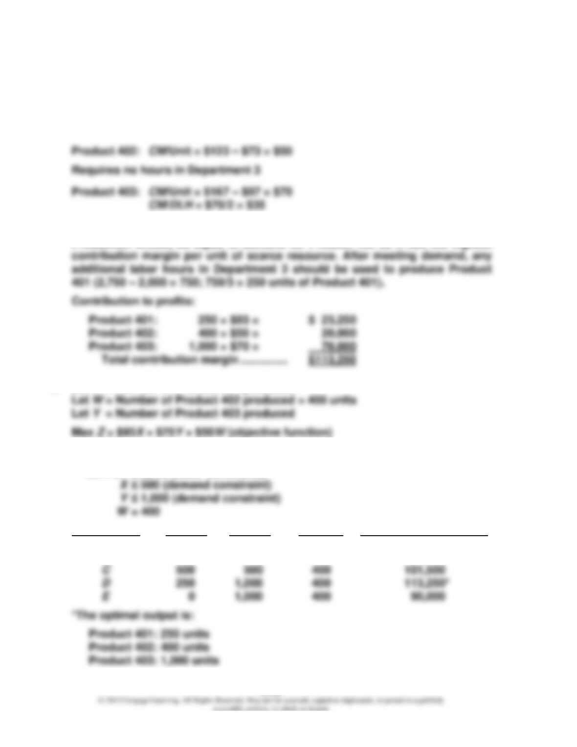
1. Dept. 1 Dept. 2 Dept. 3 Total
Product 401 (500 units):
Labor hoursa…………………. 1,000 1,500 1,500 4,000
Machine hoursb …………….. 500 500 1,000 2,000
Product 402 (400 units):
Labor hoursc…………………. 400 800 — 1,200
a2 × 500; 3 × 500; 3 × 500 d1 × 400; 1 × 400
b1 × 500; 1 × 500; 2 × 500 e2 × 1,000; 2 × 1,000; 2 × 1,000
20–22
Problem 20.27 (Continued)
2. Product 401: CM/Unit = $196 – $103 = $93
CM/DLH = $93/3 = $31
Direct labor hours needed (Dept. 3): 3 × 500 = 1,500
Direct labor hours needed (Dept. 3): 2 × 1,000 = 2,000
Production should be equal to demand for Product 403 as it has the highest
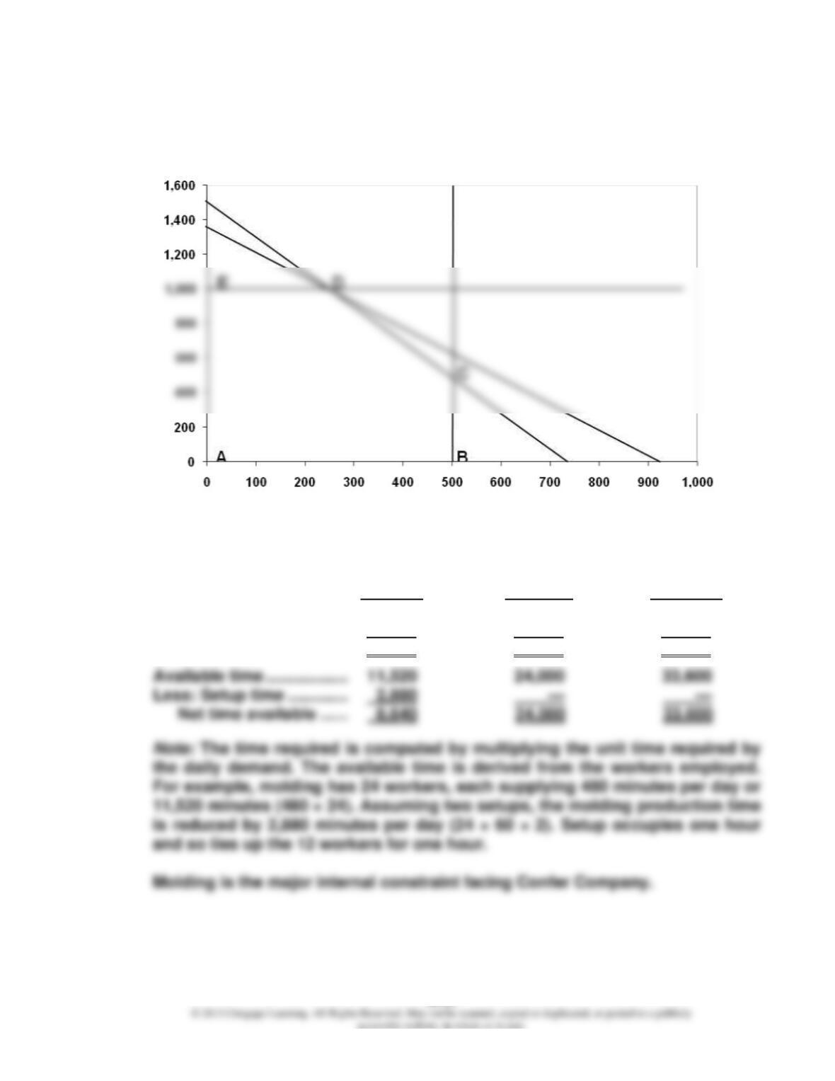
3. Let X = Number of Product 401 produced
subject to:
2X + Y ≤ 1500 (machine constraint)
3X + 2Y ≤ 2,750 (labor constraint)
Corner Point X-Value Y-Value W-Value Z = $93X + $70Y + $50W
A 0 0 400 $ 20,000
B 500 0 400 66,500
20–23
Problem 20.27 (Concluded)
At this output, the contribution to profits is $113,250.
Problem 20.28
1. Molding Grinding Finishing
Component X ………………. 3,000 6,000 9,000
Component Y ………………. 10,000 15,000 20,000
Total requirements….. 13,000 21,000 29,000
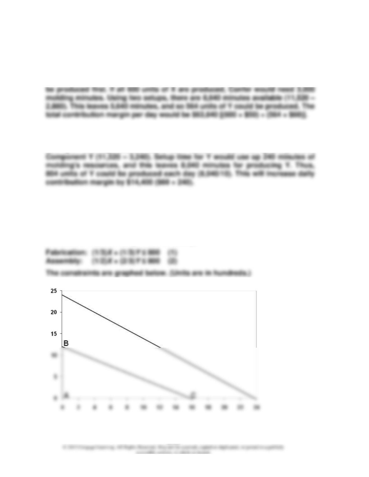
20–24
Problem 20.28 (Concluded)
2. The contribution per unit for X is $50 ($90 – $40) and for Y is $60 ($110 – $50).
The contribution margin per unit of scarce resource is $10 per minute ($50/5)
for Component X and $6 per minute ($60/10) for Component Y. Thus, X should
3. A setup time of 10 minutes would tie up the 24 workers for only 10 minutes.
Thus, production time lost is 240 minutes per setup. After setting up and pro-
ducing all of X required, this would leave 8,280 minutes to set up and produce
Problem 20.29
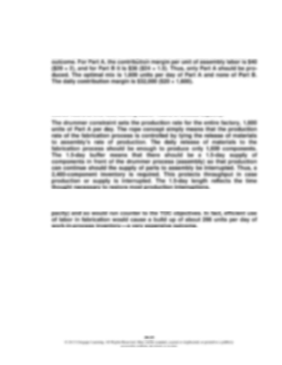
1. The constraints are both labor constraints, one for fabrication and one for as-
sembly (let X = the units of Part A and Y = the units of Part B; hours are used
to measure resource usage and availability):
Problem 20.29 (Continued)
The graph reveals that only one binding constraint is possible (assembly la-
bor). Thus, the contribution margin per unit of scarce resource will dictate the
2. The drummer constraint is the assembly constraint. The mix dictates a pro-
duction rate of 1,600 units of Part A per day. At this rate, all 800 hours availa-
ble of the drummer constraint are used. The fabrication constraint would use
533.33 hours at this rate, leaving 266.67 hours of excess capacity.
3. The use of local labor efficiency measures would encourage the fabrication
process to produce at a higher rate than the drummer rate (it has excess ca-
20–26
Problem 20.29 (Concluded)
4. Adding a second shift of 50 workers for the assembly process creates an
additional 400 hours of assembly resource. There would now be 1,200 hours
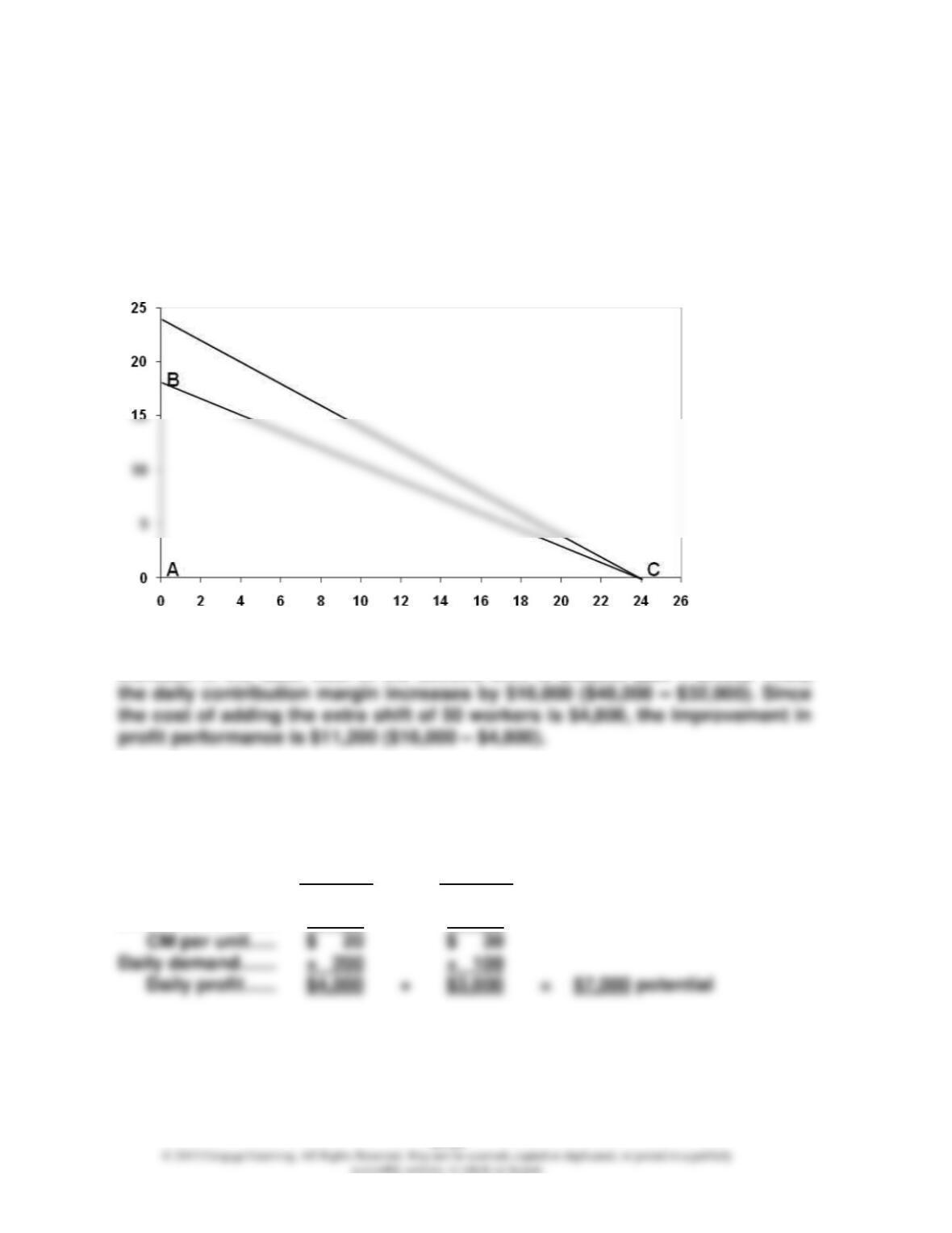
of assembly resource available. The assembly constraint now appears as
follows: (1/2)X + (2/3)Y ≤ 1,200.
The new constraint graph appears below. (Units are in hundreds.)
Point C is now optimal: X = 2,400, Y = 0. The contribution margin before the
increase in the labor cost of the second shift is $48,000 ($20 × 2,400). Thus,
Problem 20.30
1. Potential daily sales:
Frame X Frame Y
Sales ……………….. $ 40 $ 55
Materials ………….. 20 25
20–27
Problem 20.30 (Continued)
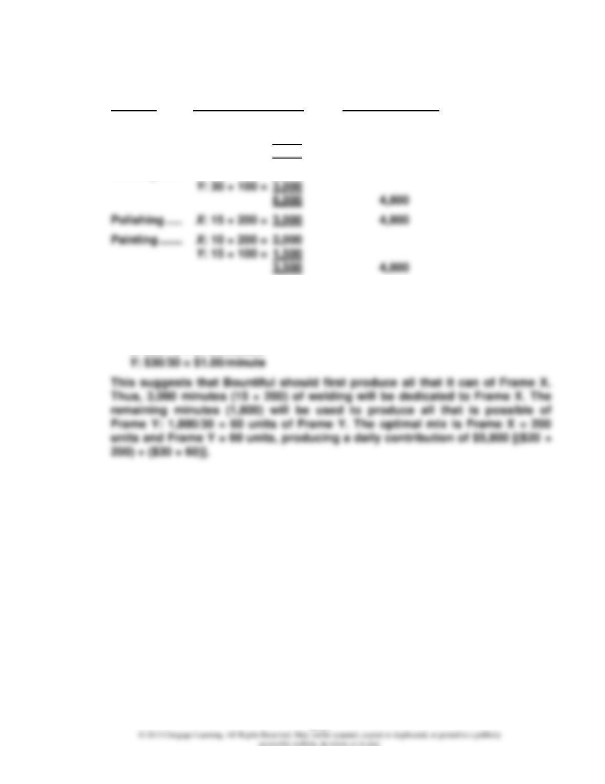
Process Resource Demands Resource Supply
Cutting ……… X: 15 × 200 = 3,000
Y: 10 × 100 = 1,000
4,000 4,800
Welding ……. X: 15 × 200 = 3,000
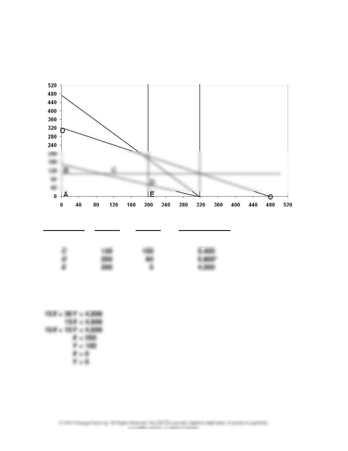
Bountiful cannot meet daily demand. The welding process requires 6,000
minutes but only has 4,800 available. All other processes have excess capaci-
ty. Thus, welding is the bottleneck. The contribution margin per unit of weld-
ing resource (minutes) for each product is computed as follows:
X: $20/15 = $1.33/minute
20–28
Problem 20.30 (Continued)
2.
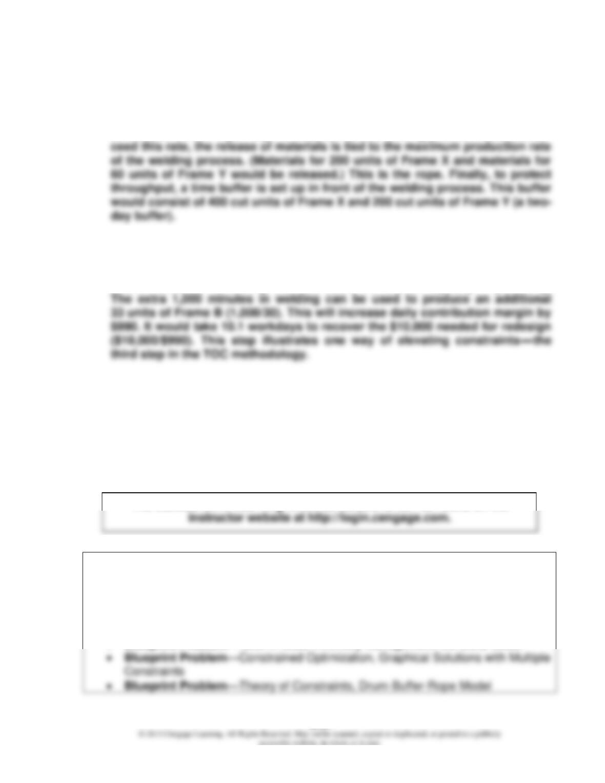
Corner Point X-Value Y-Value Z = $20X + $30Y
A 0 0 $ 0
B 0 100 3,000
*Optimal point.
Max Z = 20X + 30Y
subject to:
15X + 10Y < 4,800
20–29
Problem 20.30 (Concluded)
3. The welding process is the drummer. It sets the production rate for the entire
plant. Thus, the plant should produce 200 units of Frame X per day and
60 units of Frame Y per day. To ensure that the cutting process does not ex-
4. The redesign would increase the polishing time for Frame X from 3,000
minutes to 4,600 minutes and, at the same time, decrease the welding time for
Frame X from 3,000 minutes to 2,000 minutes. This frees up 1,000 minutes of
scarce resource in welding and decreases the excess capacity of polishing.
CYBER RESEARCH CASE
20.31
Answers will vary.
The following problems can be assigned within CengageNOW and are auto-
graded. See the last page of each chapter for descriptions of these new assign-
ments.
• Integrative Exercise—CVP, Break-Even Analysis, Theory of Constraints (Co-
vers chapters 16, 19, and 20)
• Blueprint Problem— Just-In-Case Inventory Management: the EOQ Model
The Collaborative Learning Exercise Solutions can be found on the