CHAPTER 20
INVENTORY MANAGEMENT: ECONOMIC ORDER
QUANTITY, JIT, AND THE THEORY OF CONSTRAINTS
DISCUSSION QUESTIONS
1. Ordering costs are the costs of placing and
receiving an order. Examples include clerical
costs, documents, and unloading. Setup
costs are the costs of preparing equipment
and facilities so that they can be used for
producing a product or component. Exam-
ples include wages of idled production wor-
2. As ordering costs decrease, fewer and larg-
er orders must be placed. This, in turn,
increases the units in inventory and, thus,
increases carrying costs.
3. Reasons for carrying inventory: (a) to balance
setup and carrying costs; (b) to satisfy
4. Stock-out costs are the costs of insufficient
inventory (e.g., lost sales and interrupted
production).
5. Safety stock is simply the difference between
maximum demand and average demand,
multiplied by the lead time. By re-ordering
6. The economic order quantity is the amount
of inventory that should be ordered at any
7. JIT minimizes carrying costs by driving
inventories to insignificant levels. Ordering
8. Shutdowns in a JIT environment are avoided
by practicing total preventive maintenance
and total quality control and by developing
close relationships with suppliers to ensure
on-time delivery of materials. Internally, a
Kanban system is used to ensure the timely
flow of materials and components.
9. The Kanban system is used to ensure that
10. JIT hedges against future price increases
and obtains lower input prices (better usually
than quantity discounts) by the use of long–
term contractual relationships with suppliers.
Suppliers are willing to give these breaks so
that they can reduce the uncertainty in the
demand for their products.
straints are limiting factors imposed on the
firm from external sources.
12. First, graph all constraints. Second, identify
the corner points of the feasible region.
Third, compute the value of the objective
function for each corner point. Fourth, the
used to solve higher dimensional linear pro-
gramming problems.
ization generates money through sales.
(2) Inventory—the money an organization
spends in turning materials into throughput.
spends).
20-2
14. Lower inventories mean that a company
must pay attention to higher quality —it
cannot afford to have production go down
because of defective parts or products. It
15. (1) Identify constraints, (2) exploit binding
constraints, (3) subordinate everything else
to decisions made in step 2, (4) elevate
binding constraints, and (5) repeat.
20-3
CORNERSTONE EXERCISES
Cornerstone Exercise 20.1
1. Number of orders = D/Q = 12,500/250 = 50. Ordering cost = P × D/Q = $45 × 50
= $2,250.
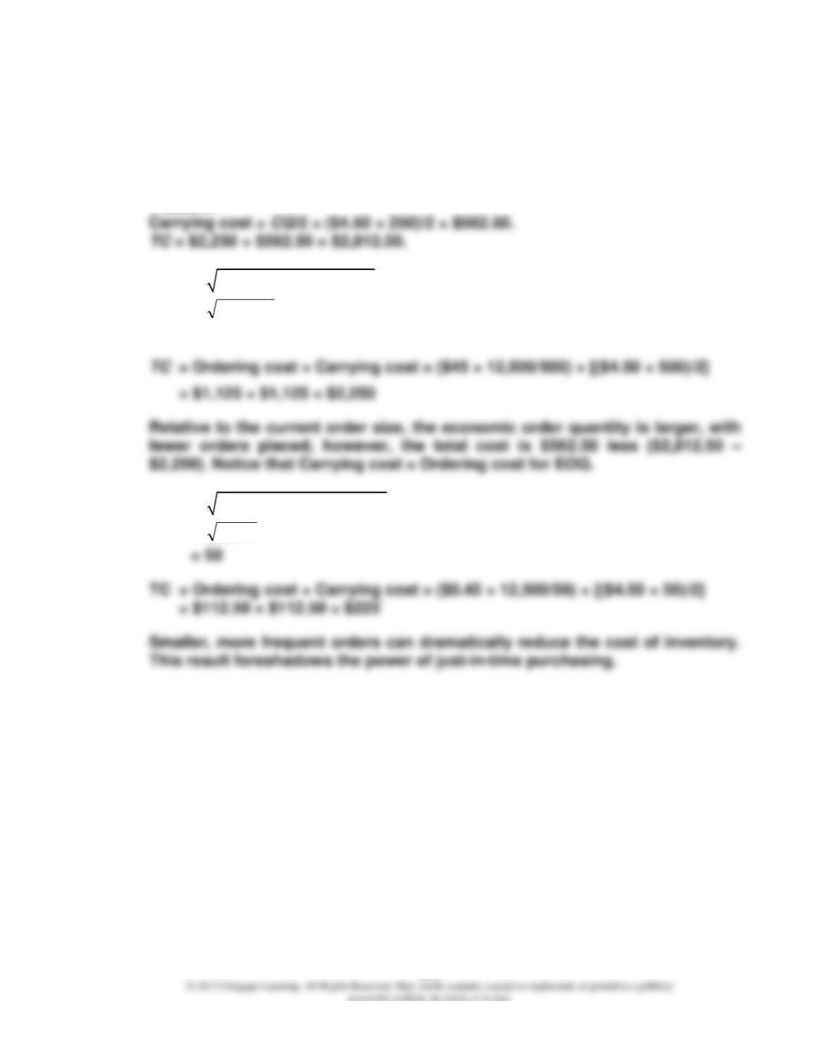
2. EOQ =
( )
2×12,500× $45 /$4.50
=
000,250
= 500
3. EOQ =
( )
2×12,500×$0.45 /$4.50
=
500,2
20-4
Cornerstone Exercise 20.2
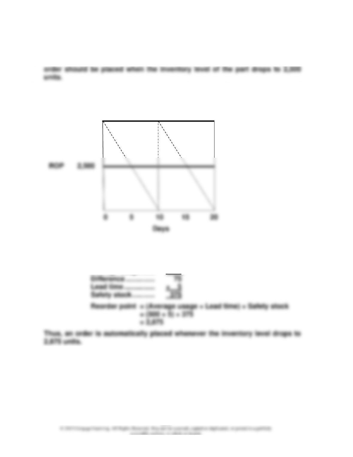
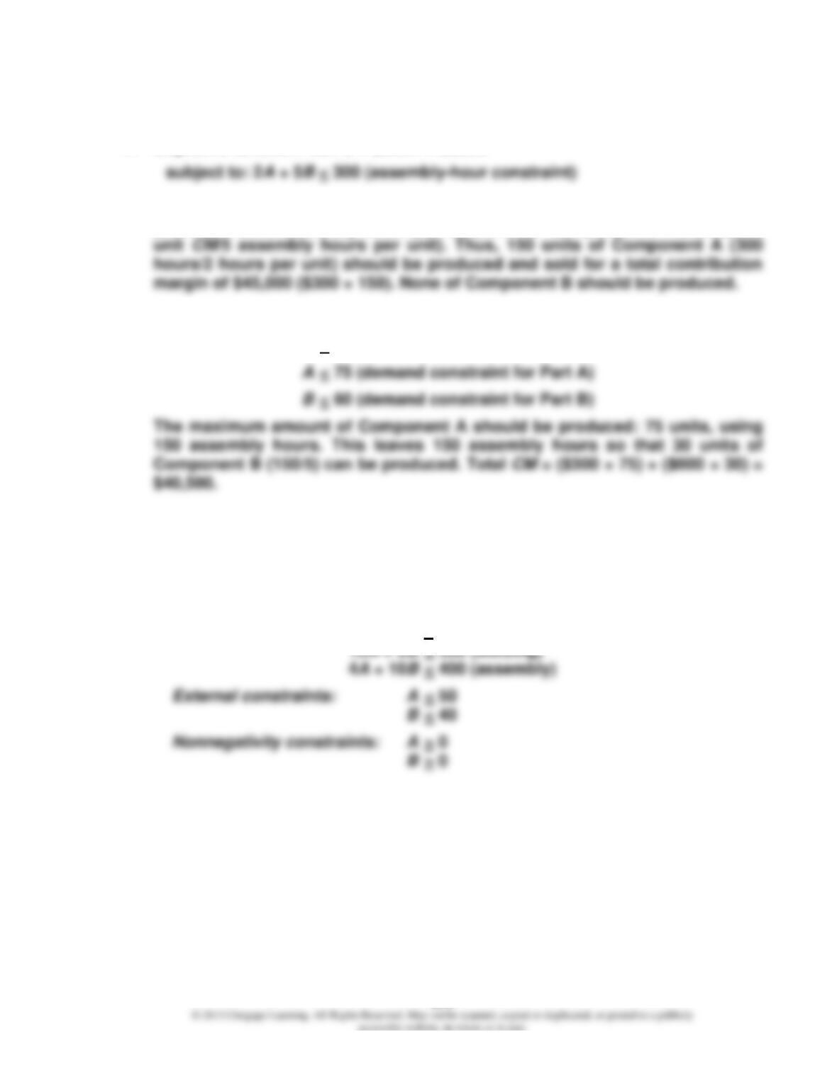
1. Reorder point = Rate of usage × Lead time = 500 × 5 = 2,500 units. Thus, an
2. The inventory is depleted just as the order arrives. The quantity on hand
jumps back up to the EOQ level.
Inventory (units)
3. With uncertainty, safety stock is needed. Safety stock is computed as follows:
Maximum usage ….. 575
Average usage ……. (500)
EOQ 5,000
20-5
Cornerstone Exercise 20.3
1. Objective function: Max Z = $300A + $600B
2. Contribution margin (CM) per unit of scarce resource for Component A = $150
($300 unit CM/2 assembly hours per unit) and for Component B = $120 ($600
3. Max Z = $300A + $600B
subject to: 2A + 5B < 300 (assembly-hour constraint)
Cornerstone Exercise 20.4
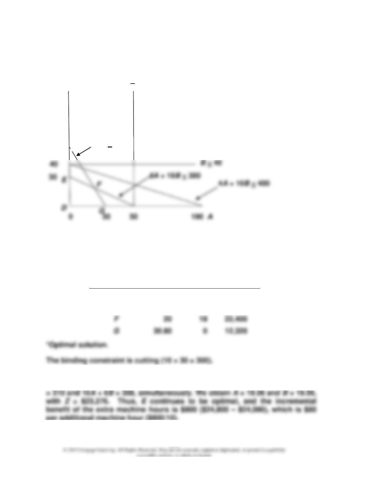
1. Max Z = $400A + $600B
subject to:
Internal constraints: 6A + 10B < 300 (cutting)
20-6
Cornerstone Exercise 20.4 (Concluded)
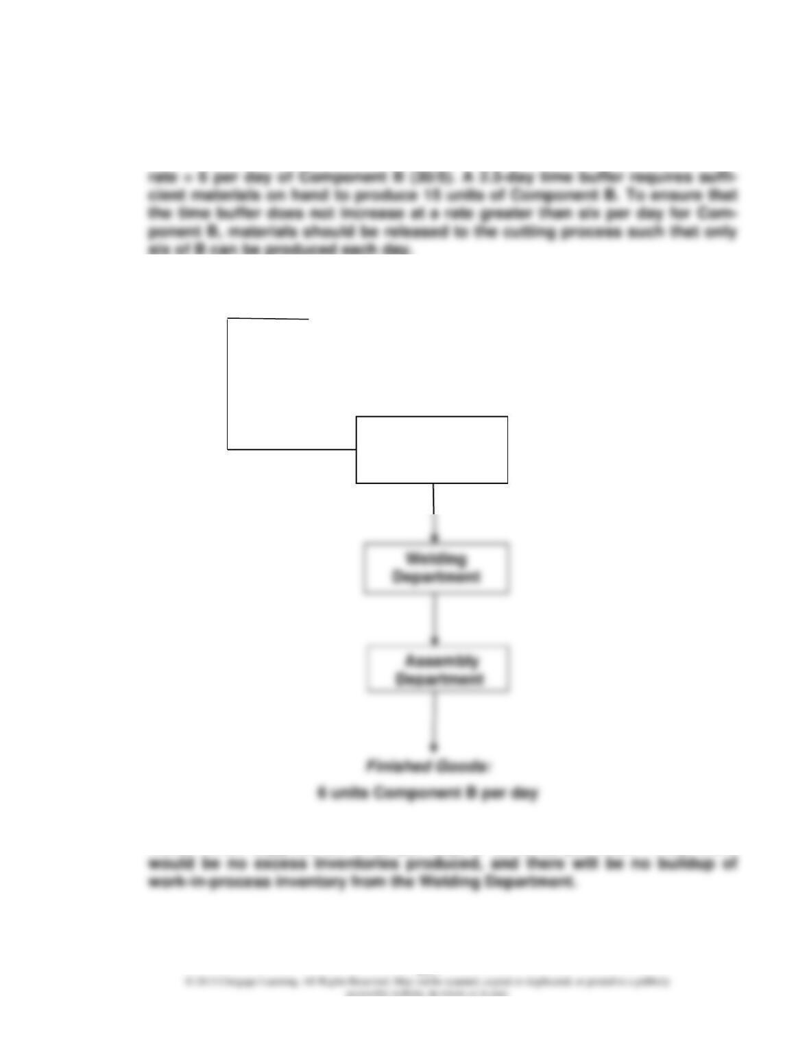
2. The graph of the constraint set is:
B 100
The coordinates of D, E, F, and G are obtained by solving the simultaneous
equations of the associated intersecting constraints that define the feasible
set (Region DEFG).
Corner Point
A-Value
B-Value
Z = $400A +
$800B
D
0
0
$
0
E
0
30
24,000
*
22,400
G
30.80
0
12,320
3. The feasible corner points affected are E and F. E now has coordinates (0,
31); thus, Z = $24,800. For F, the coordinates are obtained by solving 6A + 10B
A < 50
50
10A + 6B < 308
20-7
Cornerstone Exercise 20.5
1. Binding constraint: cutting. Since there is only one binding constraint, this
constraint becomes the drummer. Thus, cutting is the drummer. Production
2.
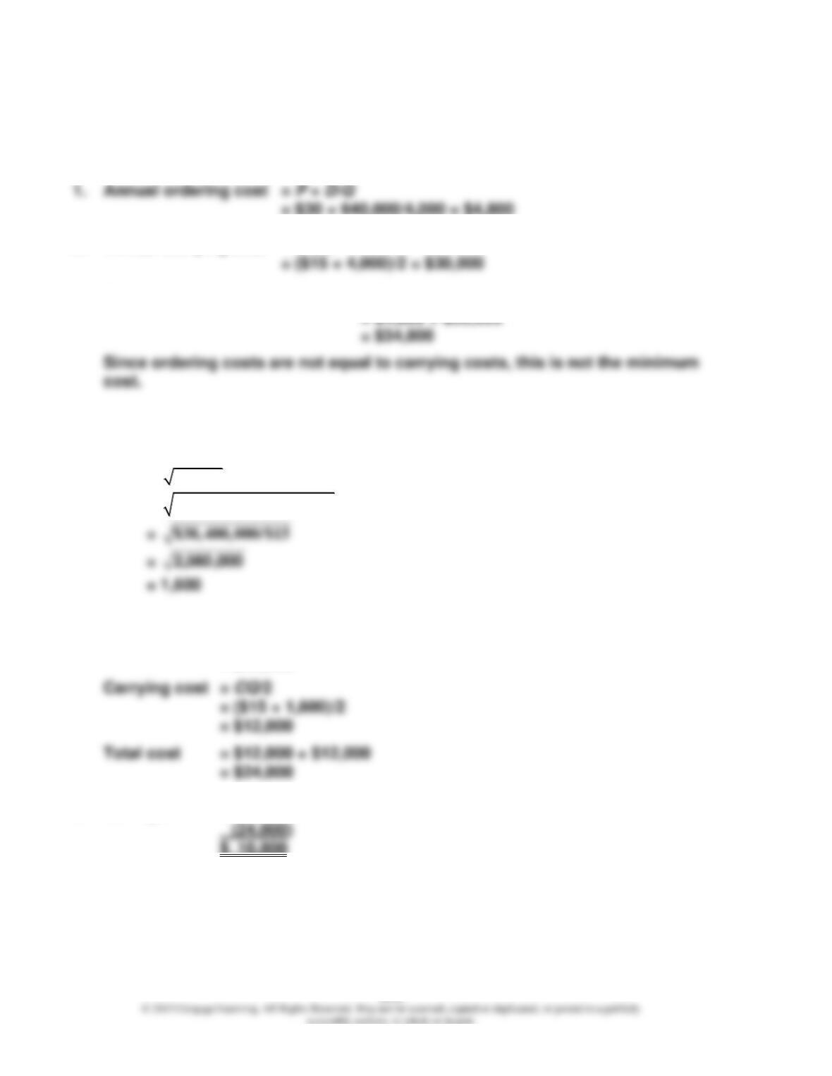
Rope: Materials for six units of Component B per day:
3. The Welding Department cannot produce any faster than the Cutting Depart-
ment, which supplies six units per day, or 30 units per week. Thus, there
Drummer:
Cutting
Department
Time Buffer:
Materials for 15 units of
Component B
20-8
EXERCISES
Exercise 20.6
2. Annual carrying cost = CQ/2
3. Cost of current inventory policy = Ordering cost + Carrying cost
Exercise 20.7
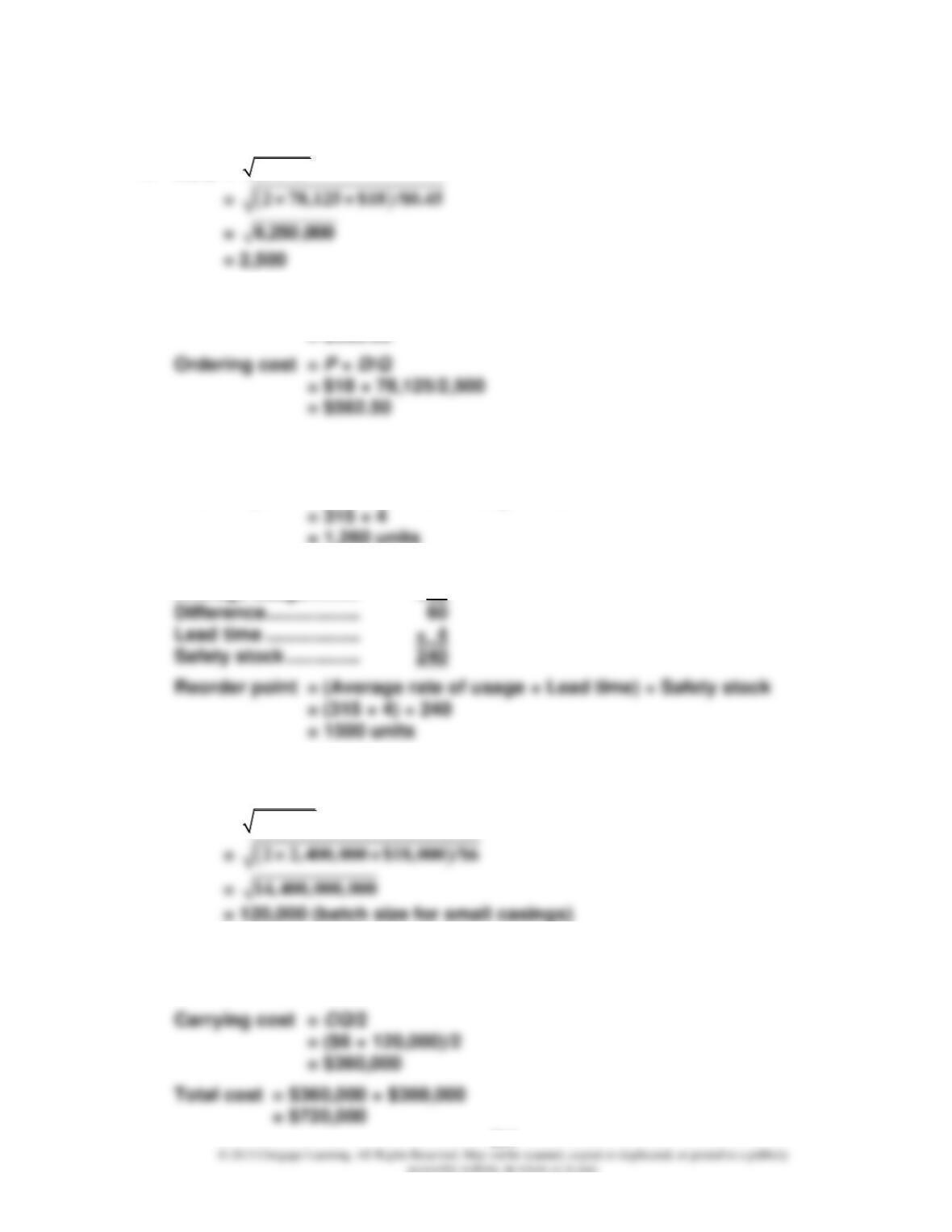
1. EOQ =
2DP/C
=
( )
2 × 640,000 × $30 /$15
2. Ordering cost = P × D/Q
= $30 × 640,000/1,600
= $12,000
3. Savings: $ 34,800
20-9
Exercise 20.8
1. EOQ =
2DP/C
2. Carrying cost = CQ/2
= ($0.45 × 2,500)/2
= $562.50
Exercise 20.9
1. Reorder point = Average rate of usage × Lead time
2. Maximum usage ……. 375
Average usage ………. 315
Exercise 20.10
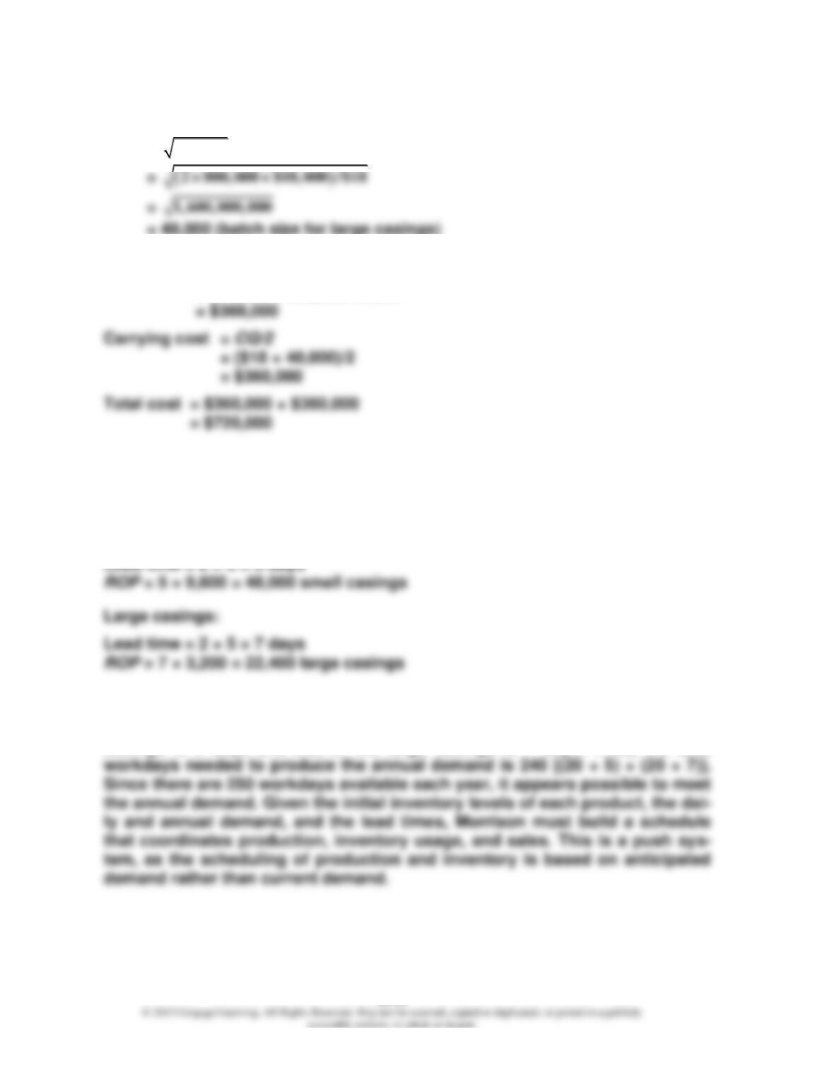
1. EOQ =
2DP / C
2. Setup cost = P × D/Q
= $18,000 × 2,400,000/120,000
= $360,000
20–10
Exercise 20.11
1. EOQ =
2DP / C
2. Setup cost = P × D/Q
= $18,000 × 800,000/40,000
Exercise 20.12
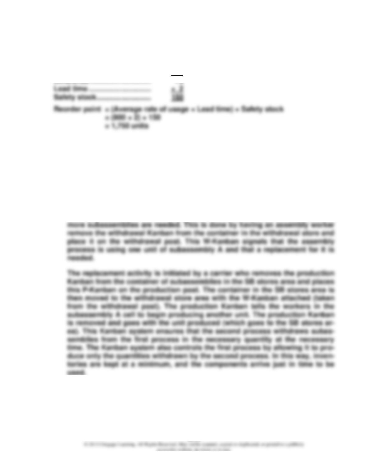
1. Small casings:
ROP = Lead time × Average daily sales
2. Small casings require 20 batches per year (2,400,000/120,000). Large casings
also require 20 batches per year (800,000/40,000). The lead time for the small
casings is 5 days and that of the large casings is 7 days. Thus, the total
20–11
Exercise 20.13
Maximum daily usage ……….. 875
Average daily usage …………. 800
Exercise 20.14
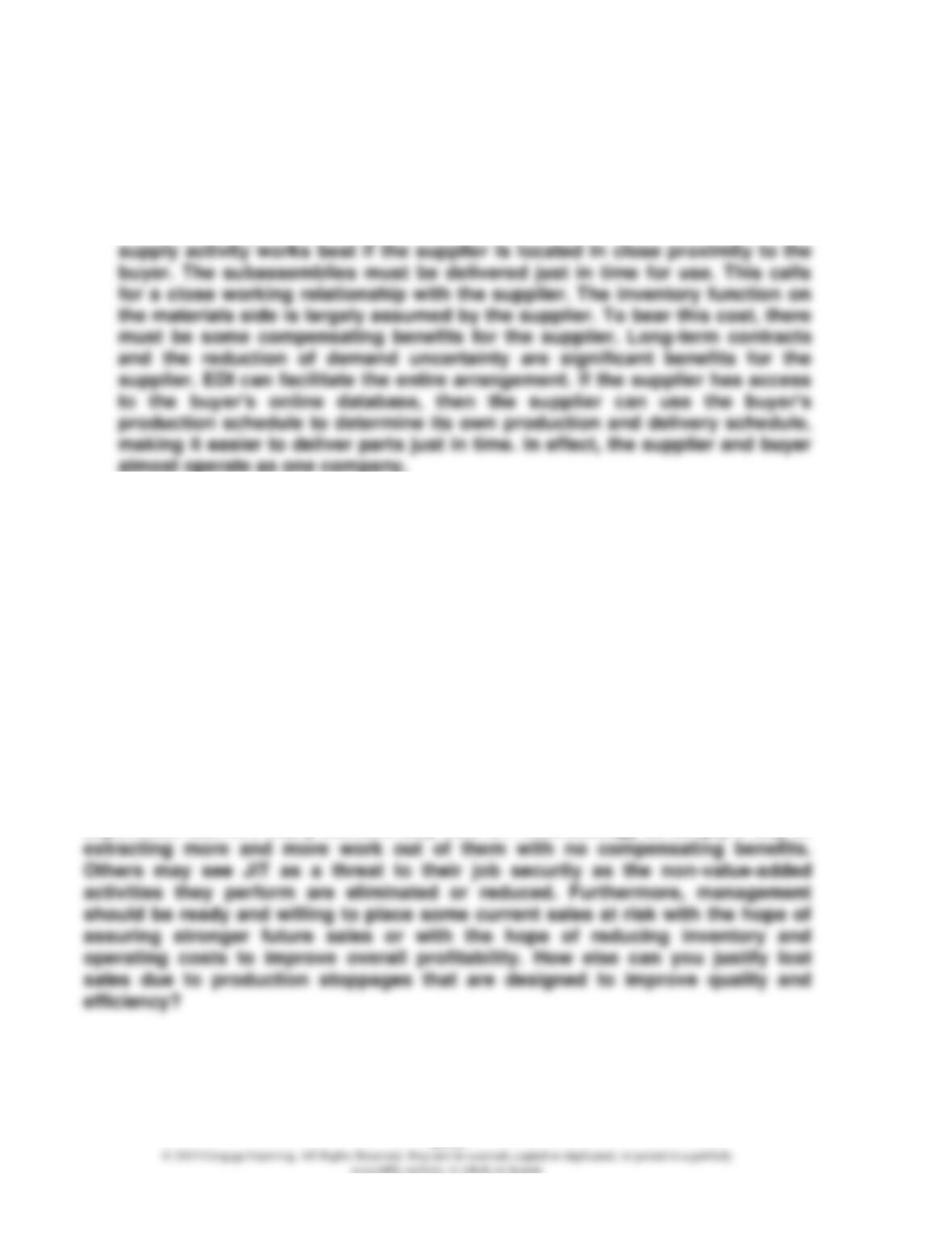
1. The entire Kanban cycle begins with the need to produce a final product—a
product demanded by a customer. The demand for a product to be assembled
is known from the production schedule. Assume that a final product is need-
ed. The withdrawal Kanban controls movement of work between the assembly
process and the manufacturing processes. It specifies the quantity that a
subsequent process should withdraw from the preceding process. The as-
sembly process uses withdrawal Kanbans to notify the first process that
20–12
Exercise 20.14 (Concluded)
2. The second process uses a vendor Kanban to signal the supplier that another
order is needed. The process is similar to the internal flow described in
Requirement 1. However, for the process to work with suppliers, the suppliers
must be willing to make frequent and small deliveries. It also means that the
Exercise 20.15
The phrase “implementing JIT” conveys to many the notion that one day a
company is conventional and the next day it is JIT with all of the benefits that are
typically assigned to JIT. In reality, changing to a JIT environment takes time and
patience. It is more of an evolutionary process than a revolutionary process. It
takes time to build a “partners–in–profits” relationship with suppliers. Many firms
attempt to force the JIT practice with suppliers by dictating terms—but this
approach really runs counter to the notion of developing close relationships—
something that is vital for the JIT purchasing side to work. There must be trust
and mutual benefits—not unilateral benefits—for JIT purchasing to become a
success.
Also, management should be aware of the disequilibrium that workers may
experience with JIT. Many workers may view JIT methodology as simply a way of
Exercise 20.16
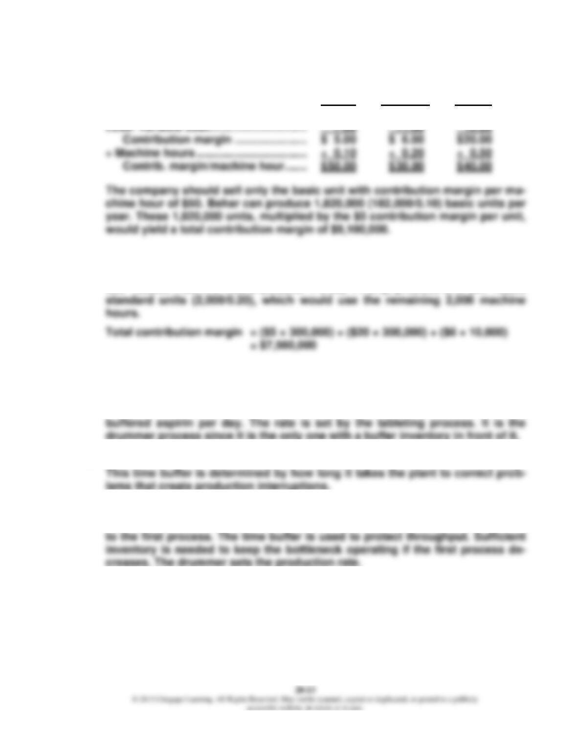
1. Basic Standard Deluxe
Price ……………………………………………… $ 12.00 $ 17.00 $ 32.00
2. Produce and sell 300,000 basic units, which would use 30,000 machine hours
(300,000 × 0.10). Next, produce and sell 300,000 deluxe units, which would
use 150,000 machine hours (300,000 × 0.50). Finally, produce and sell 10,000
Exercise 20.17
1. The production rate is 1,500 bottles of plain aspirin per day and 500 bottles of
2. Duckstein has 0.5 day of buffer inventory (1,000 bottles/2,000 bottles per day).
3. A is the rope, B is the time buffer, and C is the drummer constraint. The rope
ties the production rate of the drummer constraint to the release of materials
20–14
CPA-TYPE EXERCISES
Exercise 20.18
b. An increase in the cost of carrying inventory would lead to a reduction in av-
erage inventory. Suppose item A is required to be refrigerated so that it will
Exercise 20.19
b. Ordering cost = carrying cost for EOQ. There is not sufficient information to
Exercise 20.20
a. The best definition of EDI is electronic (computer-to-computer) exchange of
Exercise 20.21
d. For TOC, the drummer constraint sets the production rate of the factory.
Succeeding operations of necessity must match the production rate of the
Exercise 20.22
b. For a TOC setting, Encapsulating is the drummer and sets the production rate
20–15
PROBLEMS
Problem 20.23
1. EOQ =
2DP / C
=
( )
2 × 36,000 × $6,000 /$3
2. To have met the order’s requirements, Bateman could have produced 3,750
units within the seven-workday window [(7 – 2) × 750] and would have needed
8,250 units in stock—5,250 more than available. To solve delivery problems
such as the one described would likely require much more inventory than is
currently carried. If the maximum demand is predictable, then safety stock
3. EOQ =
2DP / C
=
( )
2× 36,000× $94 /$3
At a production rate of 2,000 units per day, Bateman could have satisfied the
customer’s time requirements in less than seven days—even without any
finished goods inventory. This illustrates that inventory may not be the solu-
tion to meeting customer needs or dealing with demand uncertainty. Paying