
CHAPTER 20
INVENTORY MANAGEMENT: ECONOMIC ORDER QUANTITY, JIT, AND THE THEORY
OF CONSTRAINTS
Inventory represents a significant investment of capital for most companies. Inventory management is
fundamental to establishing a long-term competitive advantage. The focus of this chapter is how
inventory policy can be used to aid in establishing a competitive advantage. Three approaches to
managing inventory are addressed: just-in-case, JIT, and theory of constraints.
LEARNING OBJECTIVES
After studying Chapter 20, students should be able to:
1. Describe the just-in-case inventory management model.
2. Discuss just-in-time (JIT) inventory management.
3. Explain the basic concepts of constrained optimization.
4. Define the theory of constraints, and tell how it can be used to manage inventory.
KEY TOPICS
The following major topics are covered in this chapter (related learning objectives are listed for each
topic):
1. Just-in-Case Inventory Management (LO 1)
2. JIT Inventory Management (LO 2)
3. Basic Concepts of Constrained Optimization (LO 3)
4. Theory of Constraints (LO 4)
I. JUST-IN-CASE INVENTORY MANAGEMENT
Inventory management is concerned with managing inventory costs. Three types of inventory costs can be
readily identified with inventory:
1. The cost of acquiring inventory
2. The cost of holding inventory
3. The cost of not having inventory on hand when needed
Ordering costs are the costs of placing and receiving an order. Examples include the costs of processing
an order (clerical costs and documents), insurance for shipment, and unloading costs. Setup costs are the
costs of preparing equipment and facilities so they can be used to produce a particular product or
component. Examples are wages of idled production workers, the cost of idled production facilities (lost
income), and the cost of test runs (labor, materials, and overhead).
Carrying costs are the costs of holding inventory. Examples include insurance, inventory taxes,
obsolescence, the opportunity cost of funds tied up in inventory, handling costs, and storage space.
Stock-out costs are the costs of not having a product available when demanded by a customer. Examples
are lost sales (both current and future), the costs of expediting (increased transportation charges, overtime,
etc.), and the costs of interrupted production.
A. Justifying Inventory
Traditional reasons for carrying inventory include:
1. To balance ordering or setup costs and carrying costs
2. Demand uncertainty
3. Machine failure
4. Defective parts
5. Unavailable parts
6. Late delivery of parts
7. Unreliable production processes
8. To take advantage of discounts
9. To hedge against future price increases
Teaching hint: It may be appropriate to briefly discuss JIT concepts at this time. Students should be aware
that traditional approaches to inventory have changed greatly.
B. Economic Order Quantity: A Model for Balancing Acquisition and Carrying Costs
A firm that keeps inventory must address the following two questions:
1. How much inventory should be ordered (or produced) to minimize inventory costs?
2. When should the order be placed (or the setup done)?
Assuming that demand is known, the total ordering (or setup) and carrying cost can be described by the
following equation:
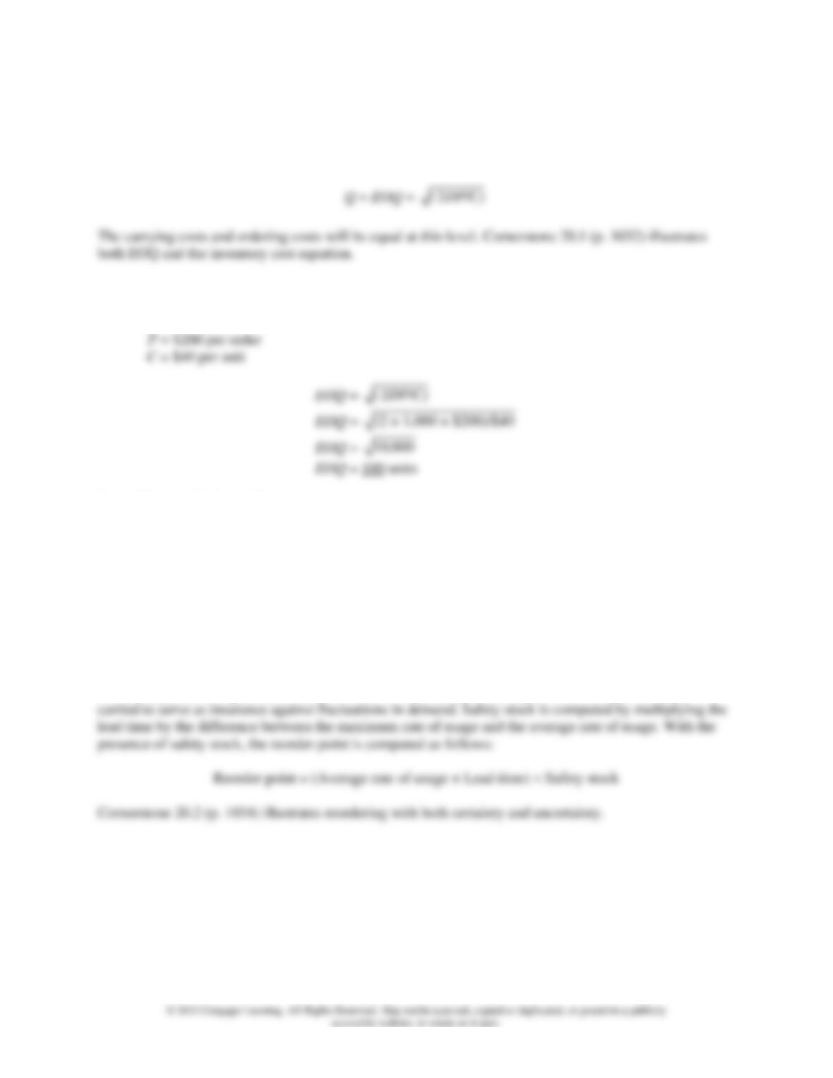
TC = PD/Q + CQ/2
= Ordering (or setup) cost + Carrying cost
where
TC = The total ordering (or setup) and carrying cost
P = The cost of placing and receiving an order (or the cost of setting up a production run)
C. Calculating EOQ
The economic order quantity (EOQ) is the amount that should be ordered (or produced) to minimize the
total ordering (or setup) costs and carrying costs. EOQ can be found using the following equation:
You can use the following information for an EOQ illustration:
D = 1,000 units
Q = 500 units
D. When to Order or Produce
The second question deals with the reorder point, which is the point in time when a new order should be
placed (or setup started). It is expressed in level of inventory: that is, when the inventory of a part reaches
a certain level, it triggers the placement of a new order. Lead time is the time required to receive the
economic order quantity once an order is placed or a setup is initiated. The reorder point is easily
computed as follows when the rate of usage is known with certainty:
Reorder point = Rate of usage × Lead time
If the demand for the part or product is not known with certainty, the possibility of stock-out exists. To
avoid this problem, organizations often choose to carry safety stock. Safety stock is extra inventory
II. JIT INVENTORY MANAGEMENT
Competitive pressures have led many firms to abandon the EOQ model in favor of a JIT approach. Just-
in-time inventory management represents the continual pursuit of productivity through the elimination of
waste. JIT has two strategic objectives: to increase profits and to improve a firm’s competitive position.
These two objectives are achieved by controlling costs (enabling better price competition and increased
profits), improving delivery performance, and improving quality. JIT offers increased cost efficiency and
simultaneously has the flexibility to respond to customer demands for better quality and more variety.
A. A Pull System
JIT maintains that goods should be pulled through the system by present demand rather than pushed
through the system on a fixed schedule based on anticipated demand.
B. Setup and Carrying Costs: The JIT/Lean Approach
JIT attempts to drive setup costs and ordering costs to zero. If those costs become insignificant, the only
remaining cost to minimize is carrying cost, which is accomplished by reducing inventories to very low
levels.
Retailers have found a way to reduce ordering costs by adopting an arrangement known as continuous
replenishment. Continuous replenishment means a manufacturer assumes the inventory management
C. Due-Date Performance: The JIT (Lean) Solution
Due-date performance is a measure of a firm’s ability to respond to customer needs. JIT solves the
problem of due-date performance by dramatically reducing lead times. Shorter lead times increase a
firm’s ability to meet requested delivery dates and to respond quickly to the demands of the market. Thus,
the firm’s competitiveness is improved. JIT cuts lead times by reducing setup times, improving quality,
and using cellular manufacturing.
D. Avoidance of Shutdown and Process Reliability: The JIT/Lean Approach
Most shutdowns occur for one of three reasons: machine failure, defective material or subassembly, and
unavailability of a material or subassembly. JIT solves these problems by emphasizing total preventive
maintenance and total quality control in addition to building the right kind of relationship with suppliers.
The Kanban system is used to ensure that parts or materials are available when needed. The Kanban
system is an information system that controls production by using markers or cards. It is responsible for
E. Discounts and Price Increases: JIT Purchasing versus Holding Inventories
To take advantage of quantity discounts and hedge against future price increases of the items purchased,
JIT negotiates long-term contracts with a few chosen suppliers located as close to the production facility
III. BASIC CONCEPTS OF CONSTRAINED OPTIMIZATION
Manufacturing and service organizations must choose the mix of products that they will produce and sell.
A manager should choose the mix alternative that maximizes total profit. Every firm will face limitations,
or constraints. External constraints are limiting factors imposed on the firm from external sources (e.g.,
A. One Binding Internal Constraint
Typically, the constrained optimization problem is modeled by (1) mathematically expressing the
objective of maximizing total contribution margin and (2) mathematically expressing both the internal
and external constraints. The function to be optimized (maximized in the case of contribution margin) is
B. Multiple Internal Binding Constraints
A linear programming model expresses a constrained optimization problem as a linear objective function
subject to a set of linear constraints. All constraints, taken together, are referred to as the constraint set. A
feasible solution is a solution that satisfies the constraints in the linear programming model. The
IV. THEORY OF CONSTRAINTS
The goal of the theory of constraints (TOC) is to make a profit now and in the future by managing
constraints. TOC recognizes that the performance of any organization is limited by its constraints. TOC
tries to identify the weakest link in a system and improve overall organizational performance by
improving the weakest link.
TOC focuses on three operational measures of systems performance: (1) throughput, (2) inventory, and
(3) operating expenses. Throughput is the rate at which an organization generates money through sales.
Inventory is all the money the organization spends in turning materials into throughput. Operating
expenses are defined as all the money the organization spends in turning inventories into throughput and,
therefore, represent all other money that an organization spends. Based on these three measures, the
objectives of management can be expressed as increasing throughput, minimizing inventory, and
decreasing operating expenses.
TOC uses five steps to achieve improved organizational performance:
1. Identify an organization’s constraints.
2. Exploit the binding constraints.
3. Subordinate everything else to the decisions made in step 2.
4. Elevate the organization’s binding constraints.
5. Repeat the process as a new constraint emerges to limit output.
The major binding constraint of an organization is defined as the drummer. The drummer constraint’s
production rate sets the production rate for the entire plant. Buffers and ropes are also used in managing
constraints to lower inventory levels and improve organizational performance. The inventory buffer is
referred to as the time buffer. A time buffer is the inventory needed to keep the constrained resource busy
for a specified time interval. Its purpose is to protect the throughput of the organization from any
disruption that can be overcome within the specified time interval. Ropes are actions taken to tie the rate
at which material is released into the plant (at the first operation) to the production rate of the constrained
resource. The objective of a rope is to ensure that the work-in-process inventory will not exceed the level
needed for the time buffer. The TOC inventory system is often called the drum-buffer-rope (DBR) system.
Exhibit 20.10 (p. 1053) illustrates the DBR structure for a general setting.
V. INFORMATION ABOUT EXERCISES, PROBLEMS, AND CASES
Exercises and problems are described below and on the following page according to coverage of content,
learning objective(s), and level of difficulty. The time required to solve the problems is roughly
proportional to the level of difficulty.
In general, basic exercises/problems are fairly simple and straightforward. The text material is relatively
brief; only one or two concepts are covered. Basic exercises and problems should take about 15 to 20
minutes each.
Moderate exercises/problems may take longer and involve more concepts. These problems may have a
“twist” and require more thought. Moderate exercises and problems may take 20 to 40 minutes each.
Challenging problems are more comprehensive and may cover more concepts. The text material is
relatively longer and may include some ambiguity. Challenging problems may take 60 to 90 minutes
each.
Cornerstone
Exercise (CS)/
Exercise/
Problem/Case
Topic
Learning
Objective
Degree of
Difficulty
CS 20.1
EOQ
LO 1
Basic
CS 20.2
Reorder Point
LO 1
Basic
Constraint

Cornerstone
Exercise (CS)/
Exercise/
Problem/Case
Topic
Learning
Objective
Degree of
Difficulty
CS 20.4
Constrained Optimization: Multiple Internal
Constraints
LO 3
Basic
CS 20.5
Drum-Buffer-Rope
LO 4
Basic
20.6
Ordering and Carrying Costs
LO 1
Basic
20.7
Economic Order Quantity
LO 1
Basic
20.8
Economic Order Quantity
LO 1
Basic
20.9
Reorder Point
LO 1
Basic
20.10
EOQ with Setup Costs
LO 1
Basic
20.11
EOQ with Setup Costs
LO 1
Basic
20.12
Reorder Point
LO 1
Basic
20.13
Safety Stock
LO 1
Basic
20.14
Kanban System, EDI
LO 2
Moderate
20.15
JIT Limitations
LO 2
Moderate
20.16
Product Mix Decision, Single Constraint
LO 3
Moderate
20.17
Drum-Buffer-Rope System
LO 4
Moderate
20.18
CPA-Type Exercise
LO 1
Basic
20.19
CPA-Type Exercise
LO 1
Basic
20.20
CPA-Type Exercise
LO 2
Basic
20.21
CPA-Type Exercise
LO 4
Basic
20.22
CPA-Type Exercise
LO 4
Basic
20.23
EOQ, Safety Stock, Lead Time, Batch Size, and JIT
LO 1, 2
Moderate
20.24
Product Mix Decisions, Multiple Constraints
LO 3
Moderate
20.25
Product Mix Decision, Single and Multiple Constraints
LO 3
Moderate
20.26
Product Mix Decision, Single and Multiple Constraints,
Basics of Linear Programming
LO 3
Moderate
20.27
Product Mix Decisions
LO 3
Moderate
20.28
Identifying and Exploiting Constraints, Constraint
Elevation
LO 4
Moderate
20.29
Theory of Constraints, Internal Constraints
LO 4
Challenging
20.30
TOC, Internal and External Constraints
LO 4
Challenging
20.31
Cyber Research Case
LO 4
Challenging
LIST OF ILLUSTRATIONS
Illustration
Topic
Exhibit 20.1
Traditional Reasons for Carrying Inventory
Exhibit 20.2
The Reorder Point
Exhibit 20.3
EOQ and Reorder Point Illustrated
Exhibit 20.4
Withdrawal Kanban
Exhibit 20.5
Production Kanban
Exhibit 20.6
Vendor Kanban
Exhibit 20.7
The Kanban Process
Exhibit 20.8
Constraint Data: Schaller Company
Exhibit 20.9
Graphical Solution
Exhibit 20.10
Drum-Buffer-Rope System: General Description

Exhibit 20.11
Drum-Buffer-Rope: Schaller Company
Exhibit 20.12
New Constraint Set: Schaller Company