Accounting Chapter 2 Homework HGT Panel Variable Sex Descriptive Statistics

2

DESCRIPTIVE

STATISTICS

2.1 We have

2.2 We have that

x

i

x



2

25

¦

2

“48.6

2

2.3 Suppose we divide the patients according to whether or not they received antibiotics, and calculate the

mean and standard deviation for each of the two subsamples:

x

sn

Antibiotics 11.57 8.81 7

CHAPTER 2/DESCRIPTIVE STATISTICS 3

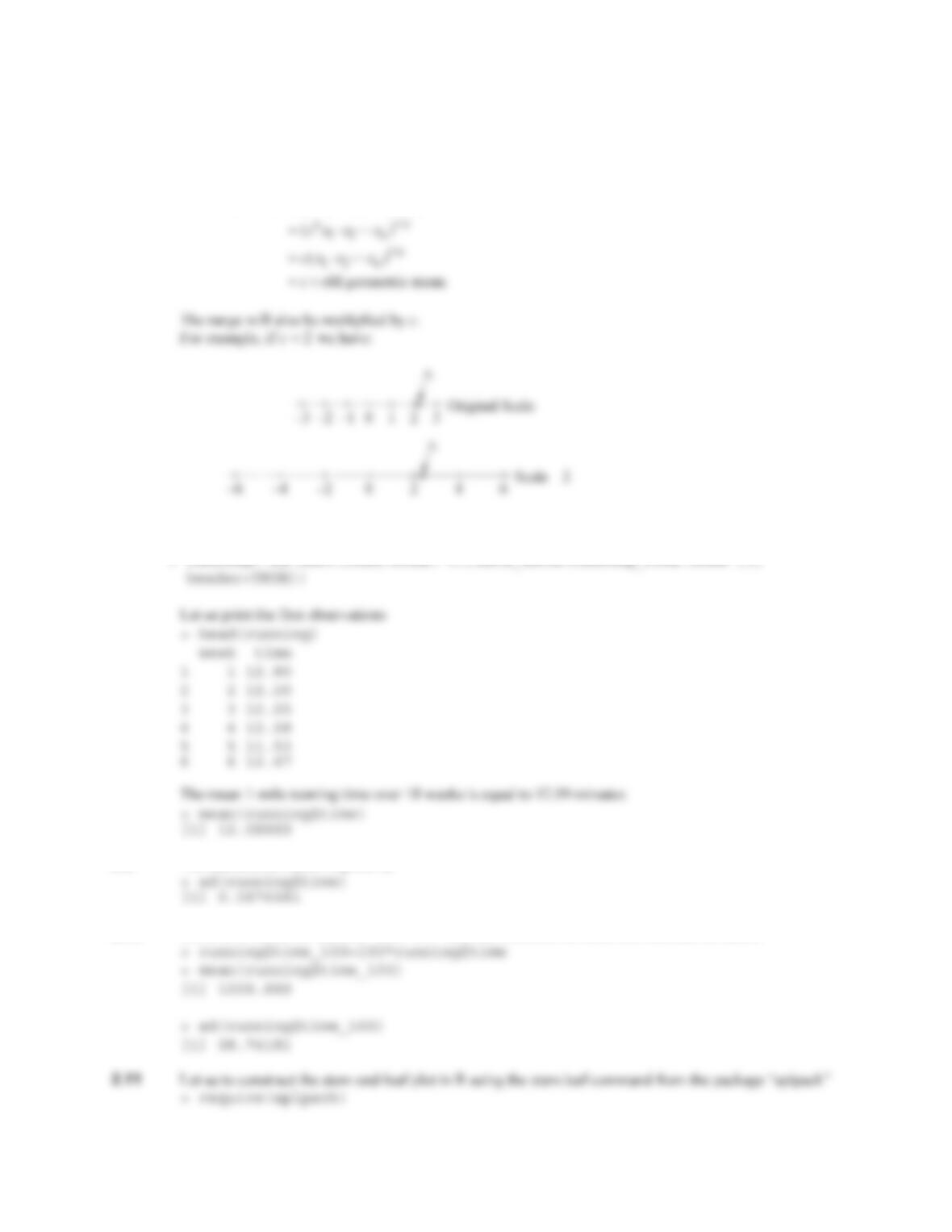
2.4-2.7 Changing the scale by a factor c will multiply each data value xi by c, changing it to cxi. Again the same

individual’s value will be at the median and the same individual’s value will be at the mode, but these

values will be multiplied by c. The geometric mean will be multiplied by c also, as can easily be shown:

Geometric mean

[( )( ) ( )]

/

cx cx cx

nn

12 1

“

2.8 We first read the data file “running time” in R

> require(xlsx)

> running<-na.omit(read.xlsx(“C:/Data_sets/running_time.xlsx”,1,

2.9 The standard deviation is given by

2.10 Let us first create the variable “time_100” and then calculate its mean and standard deviation

CHAPTER 2/DESCRIPTIVE STATISTICS 4

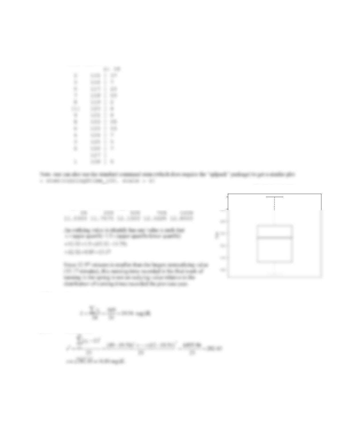
> stem.leaf(running$time_100, unit=1, trim.outliers=FALSE)

1 | 2: represents 12

leaf unit: 1

2.12 The quantiles of the running times are

> quantile(running$time)

2.13 The mean is

2.14 We have that

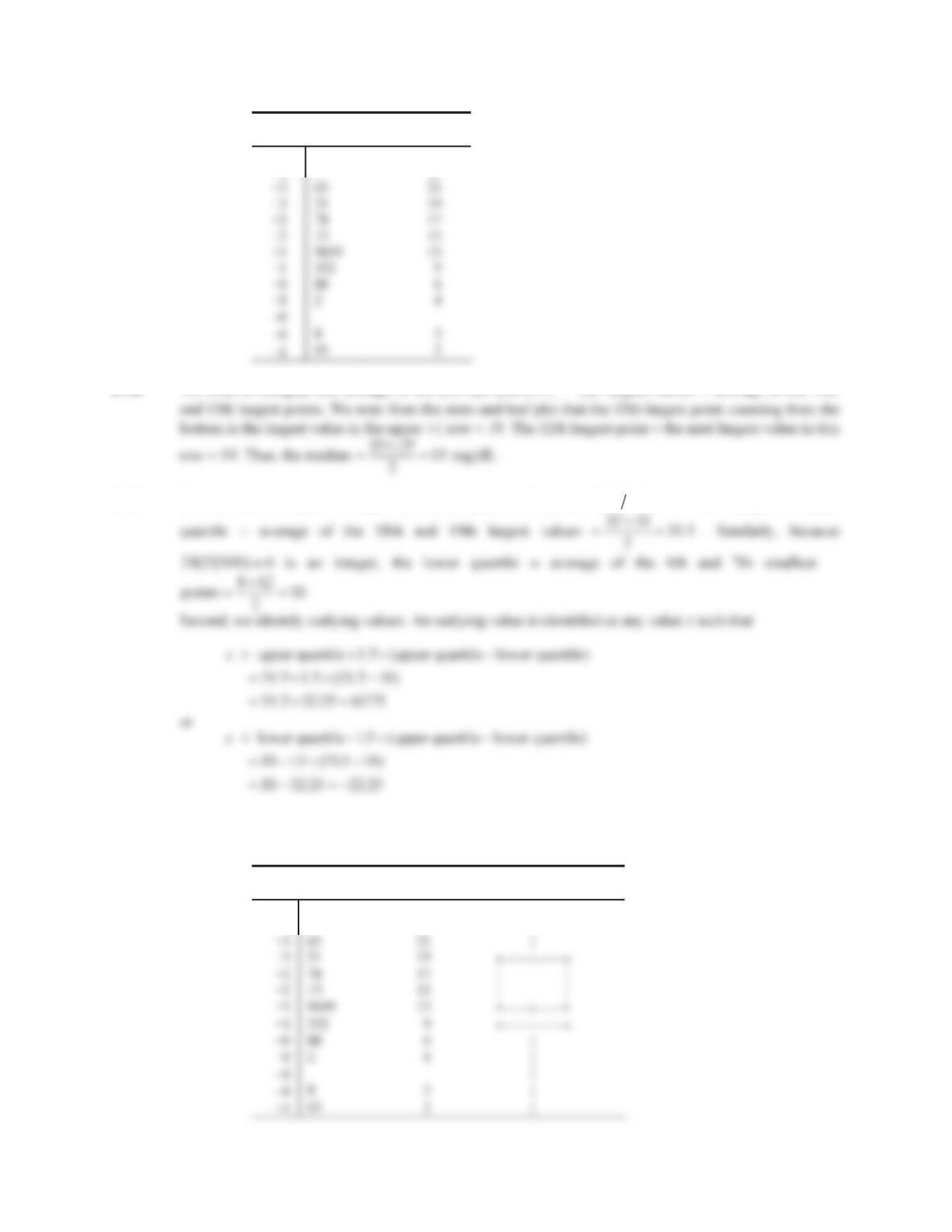
2.15 We provide two rows for each stem corresponding to leaves 5-9 and 0-4 respectively. We have

12.8

Box plot of running times

CHAPTER 2/DESCRIPTIVE STATISTICS 5

Stem-and-

leaf plot

Cumulative

frequency

+4 98 24

+4 1 22

2.16 We wish to compute the average of the (24/2)th and (24/2 + 1)th largest values average of the 12th

2.17 We first must compute the upper and lower quartiles. Because 24 75 100 18





is an integer, the upper

From the stem-and-leaf plot, we note that the range is from 13 to 49. Therefore, there are no outlying

values. Thus, the box plot is as follows:

Stem-and-

leaf plot

Cumulative

frequency Box plot

+4 98 24 |

+4 1 22 |

CHAPTER 2/DESCRIPTIVE STATISTICS 6

2.18 To compute the median cholesterol level, we construct a stem-and-leaf plot of the before-cholesterol

measurements as follows.

Stem-and-

leaf plot

Cumulative

frequency

25 0 24

24 4 23

Baseline

t179 mg/dL

Baseline

< 179 mg/dL

Stem-and-

leaf plot

Stem-and-

leaf plot

+4 98 +4

+4 +4 1

CHAPTER 2/DESCRIPTIVE STATISTICS 7

2.19 We first calculate the difference scores between the two positions:

Subject

number Subject

Systolic

difference

score

Diastolic

difference

score

1 B.R.A. 68

2 J.A.B. +2 2

11 C.R.F. +8 2

12 E.W.G. +14 +4

13 T.F.H. +2 14

Second, we calculate the mean difference scores:

21

CHAPTER 2/DESCRIPTIVE STATISTICS 8

2.20 The stem-and-leaf and box plots allowing two rows for each stem are given as follows:

Systolic Blood Pressure

Stem-and-

leaf plot

Cumulative

frequency Box plot

Diastolic Blood Pressure

Stem-and-

leaf plot

Cumulative

frequency Box plot

1 6 32 0

2.23

Id Age FEV Hgt Sex Smoke

301 9 1.708 57 0 0

451 8 1.724 67.5 0 0

CHAPTER 2/DESCRIPTIVE STATISTICS 9

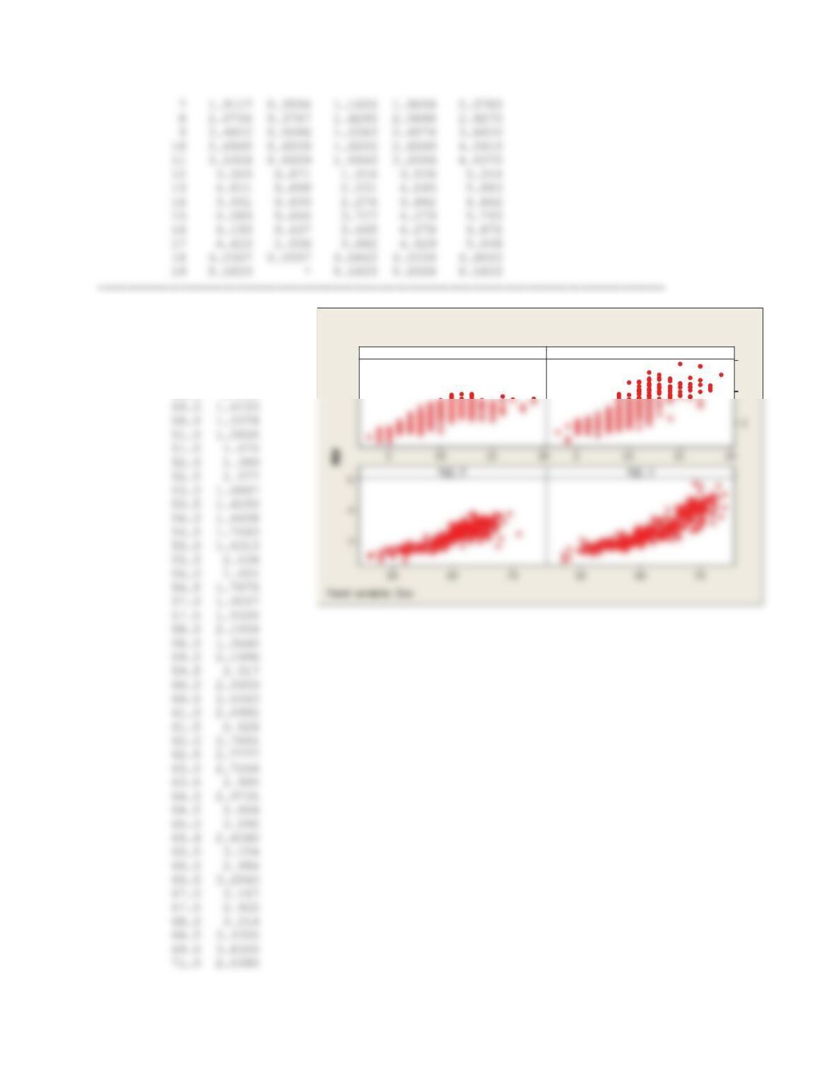
2.24 Results for Sex = 0

Variable Age Mean StDev Minimum Median Maximum

FEV 3 1.0720 * 1.0720 1.0720 1.0720

4 1.316 0.290 0.839 1.404 1.577

5 1.3599 0.2513 0.7910 1.3715 1.7040

Results for Sex = 1

Variable Age Mean StDev Minimum Median Maximum

FEV 3 1.4040 * 1.4040 1.4040 1.4040

CHAPTER 2/DESCRIPTIVE STATISTICS 10

Results for Sex = 0

Variable Hgt Mean

FEV 46.0 1.0720

46.5 1.1960

48.0 1.110

6

4

Age, 0

Age, 1

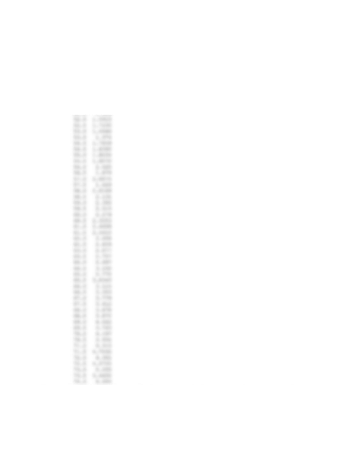
Scatterplot of FEV vs Age, Hgt

CHAPTER 2/DESCRIPTIVE STATISTICS 11

Results for Sex = 1

Variable Hgt Mean

FEV 47.0 0.981

48.0 1.270

49.5 1.4250

50.0 1.794

50.5 1.536

51.0 1.683

———-————–————–————–———–————–——–———-——–———-———-——

Descriptive Statistics: FEV

Results for Sex = 0

CHAPTER 2/DESCRIPTIVE STATISTICS 12

Results for Sex = 1

Variable Smoke Mean StDev

FEV 0 2.7344 0.9741

1 3.743 0.889

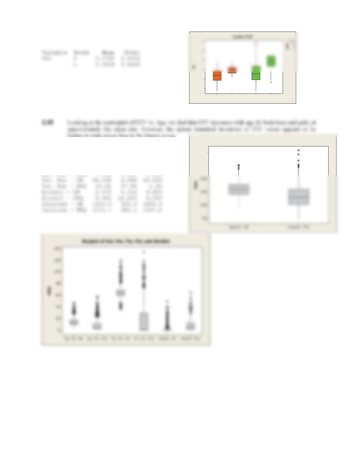
higher in male group than in the female group.

2.26

Variable Mean StDev Median

Sat. Fat – DR 14.557 7.536 12.000

2.27

Sex

Smoke

10

1010

2

1

3000

2500

Boxplot of Calories

CHAPTER 2/DESCRIPTIVE STATISTICS 13

50

120

Sat. Fat – DR*Sat. Fat – FFQ Tot. Fat – DR*Tot. Fat – FFQ

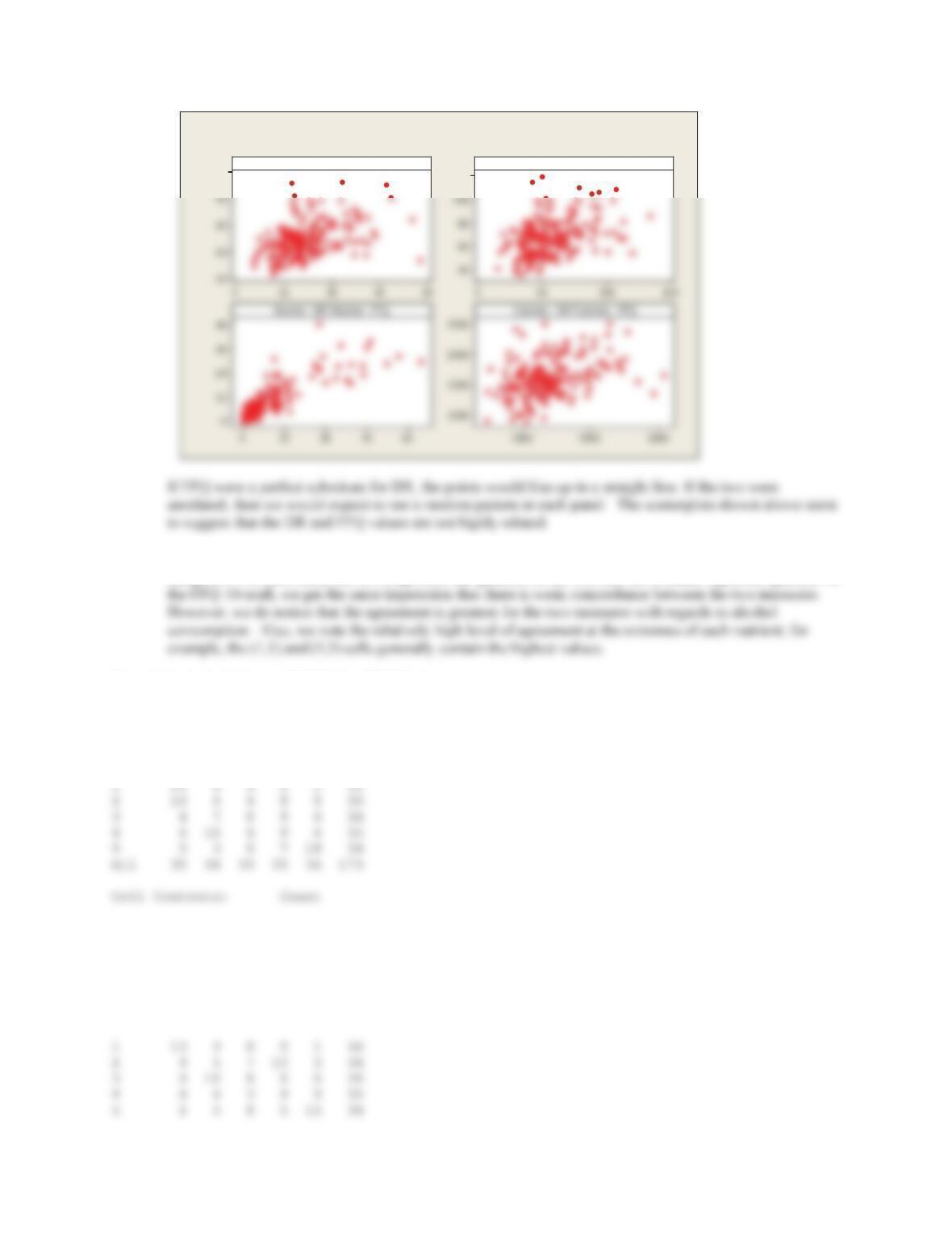
Scatterplot of DR vs. FFQ values

2.28 The 5×5 tables below show the number of people classified into a particular combination of quintile

categories. For each table, the rows represent the quintiles of the DR, and the columns represent quintiles of

Tabulated statistics: SFDQuin, SFFQuin

Rows: SFDQuin Columns: SFFQuin

1 2 3 4 5 All

Tabulated statistics: TFDQuin, TFFQuin

Rows: TFDQuin Columns: TFFQuin

1 2 3 4 5 All

CHAPTER 2/DESCRIPTIVE STATISTICS 14

Tabulated statistics: AlcDQuin, AlcFQuin

Rows: AlcDQuin Columns: AlcFQuin

1 2 3 4 5 All

Tabulated statistics: CalDQuin, CalFQuin

Rows: CalDQuin Columns: CalFQuin

1 2 3 4 5 All

2.29

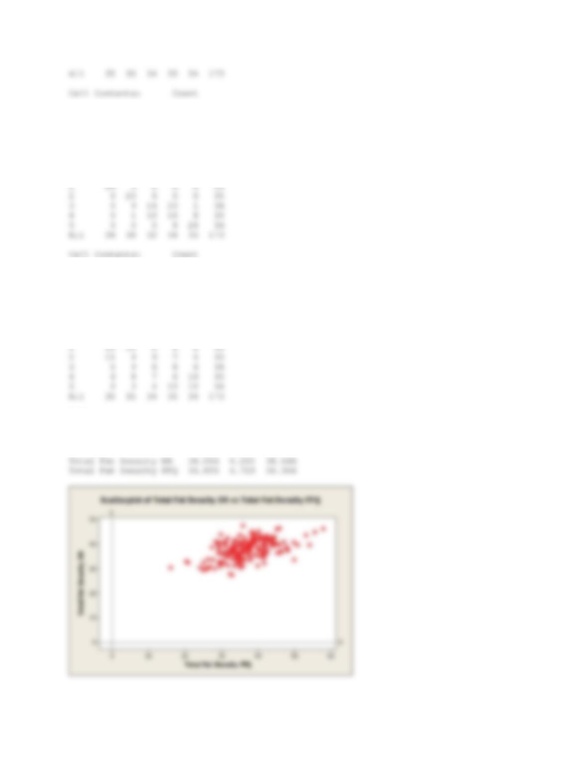
Descriptive Statistics: Total Fat Density DR, Total Fat Density FFQ

Variable Mean StDev Median

CHAPTER 2/DESCRIPTIVE STATISTICS 15

2.30 The concordance for the quintiles of nutrient density does appear somewhat stronger than for the

Tabulated statistics: Dens DR Quin, Dens FFQ Quin

Rows: Dens DR Quin Columns: Dens FFQ Quin

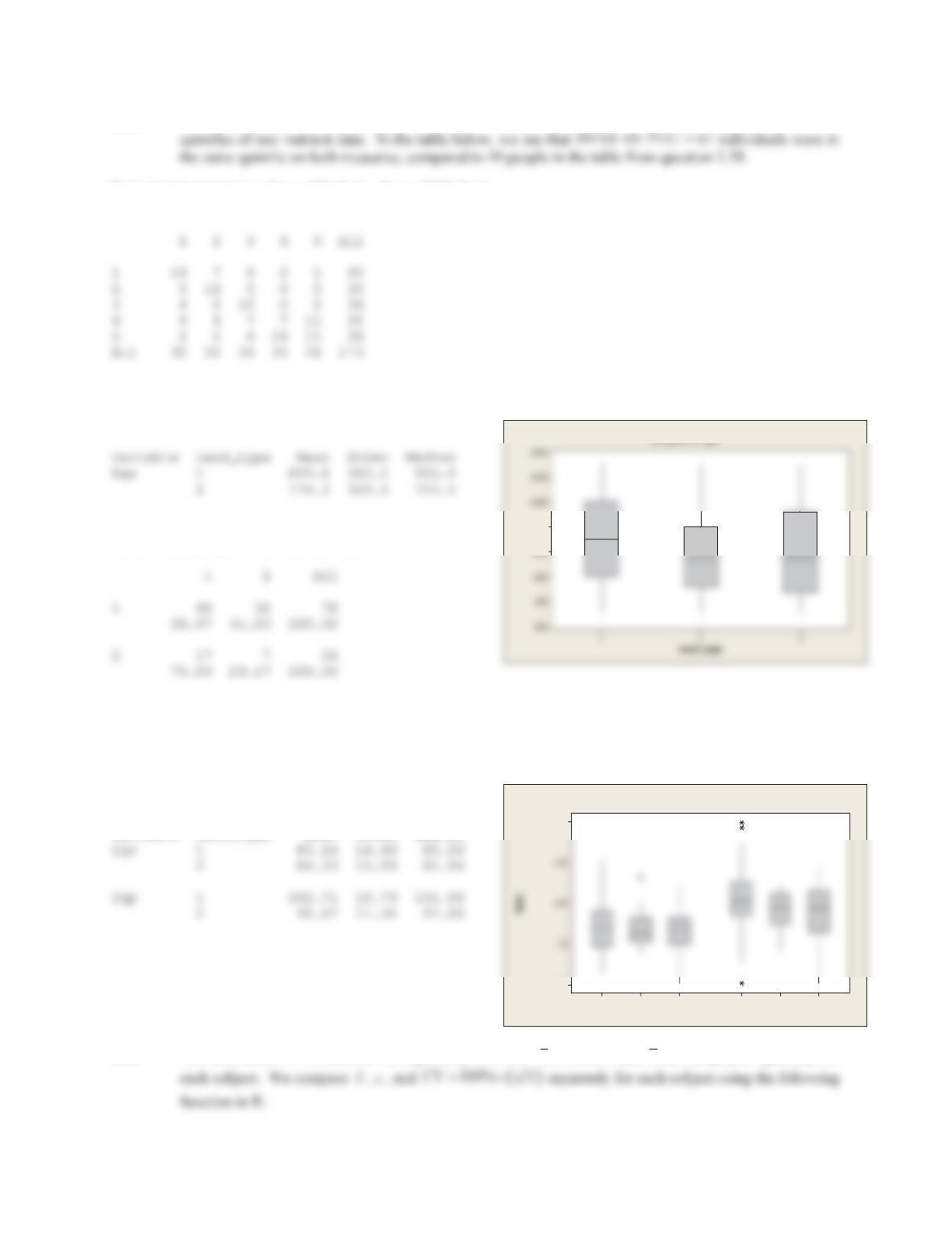
2.31 We find that exposed children (Lead type = 2) are somewhat younger and more likely to be male (Sex = 1),

compared to unexposed children. The boxplot below shows all three lead types, but we are only interested in types 1

and 2.

Tabulated statistics: Lead_type, Sex

Rows: Lead_type Columns: Sex

2.32 The exposed children have somewhat lower mean and median IQ scores compared to the unexposed

children, but the differences don’t appear to be very large.

Descriptive Statistics: Iqv, Iqp

Variable Lead_type Mean StDev Median

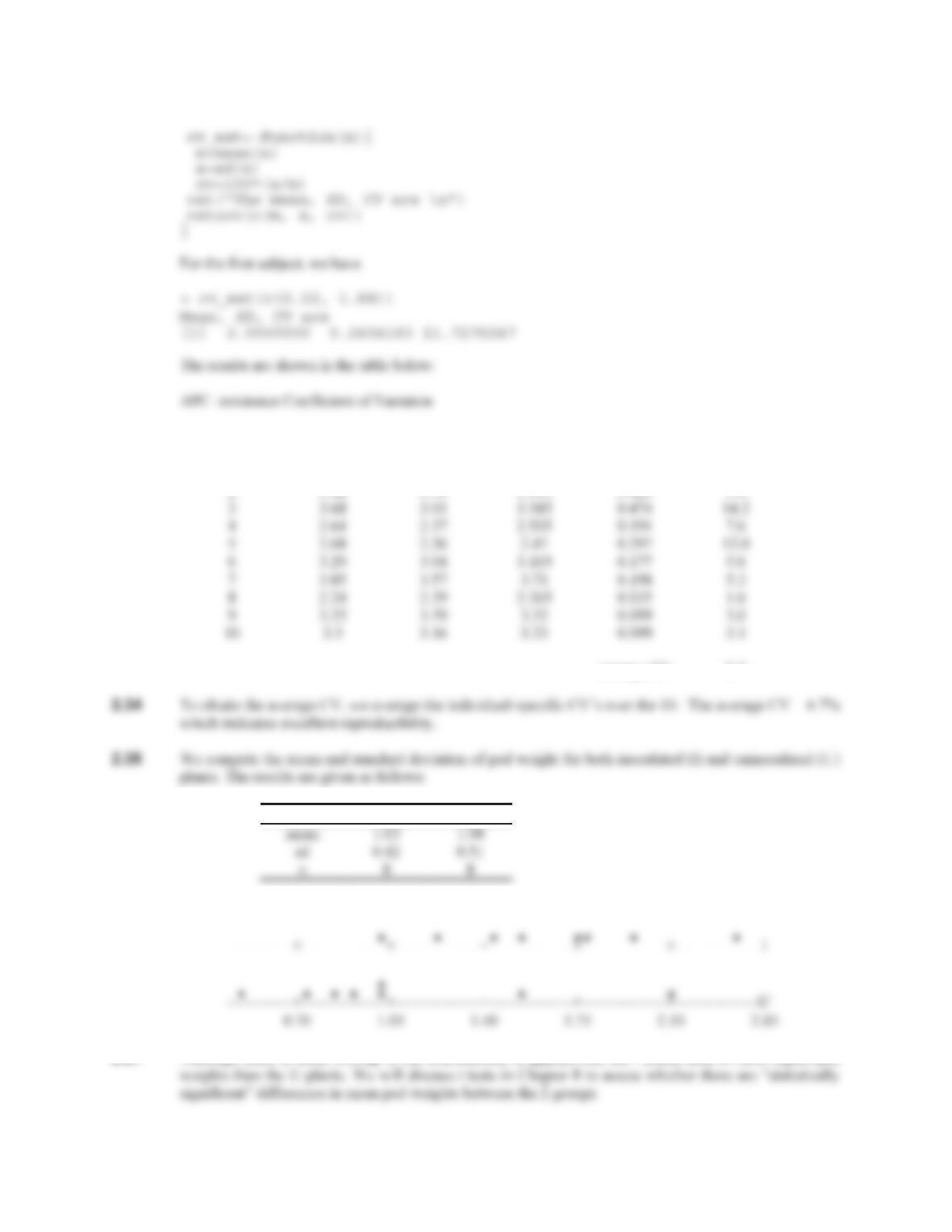
2.33 The coefficient of variation (CV) is given by 100%

s

x

/



, where s and

x

are computed separately for

1000

Age

Boxplot of Age

Lead_type

IqpIqv

321321

150

50

Boxplot of Iqv, Iqp

CHAPTER 2/DESCRIPTIVE STATISTICS 16

Sample

number A B mean sd CV

1 2.22 1.88 2.05 0.240 11.7

2 3.42 3.59 3.505 0.120 3.4

average CV 6.7

I U

2.36 We plot the distribution of I and U pod weights using a dot-plot from MINITAB.

2.37 Although there is some overlap in the distributions, it appears that the I plants tend in have higher pod

CHAPTER 2/DESCRIPTIVE STATISTICS 17

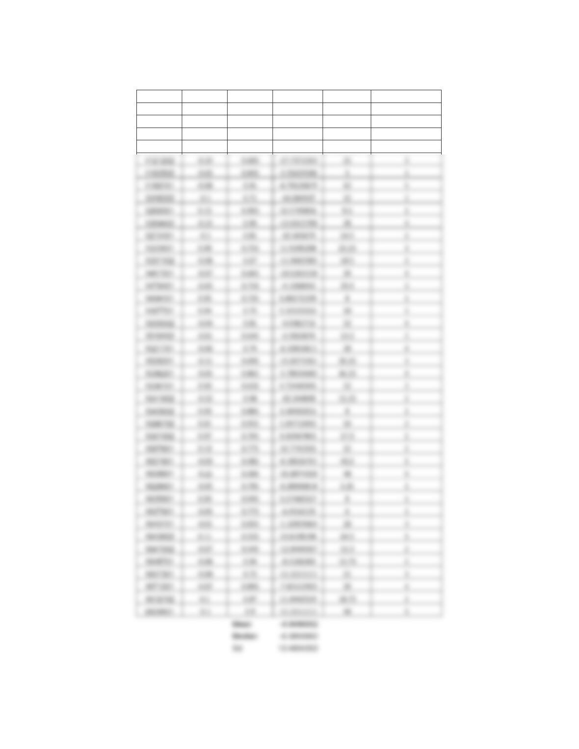
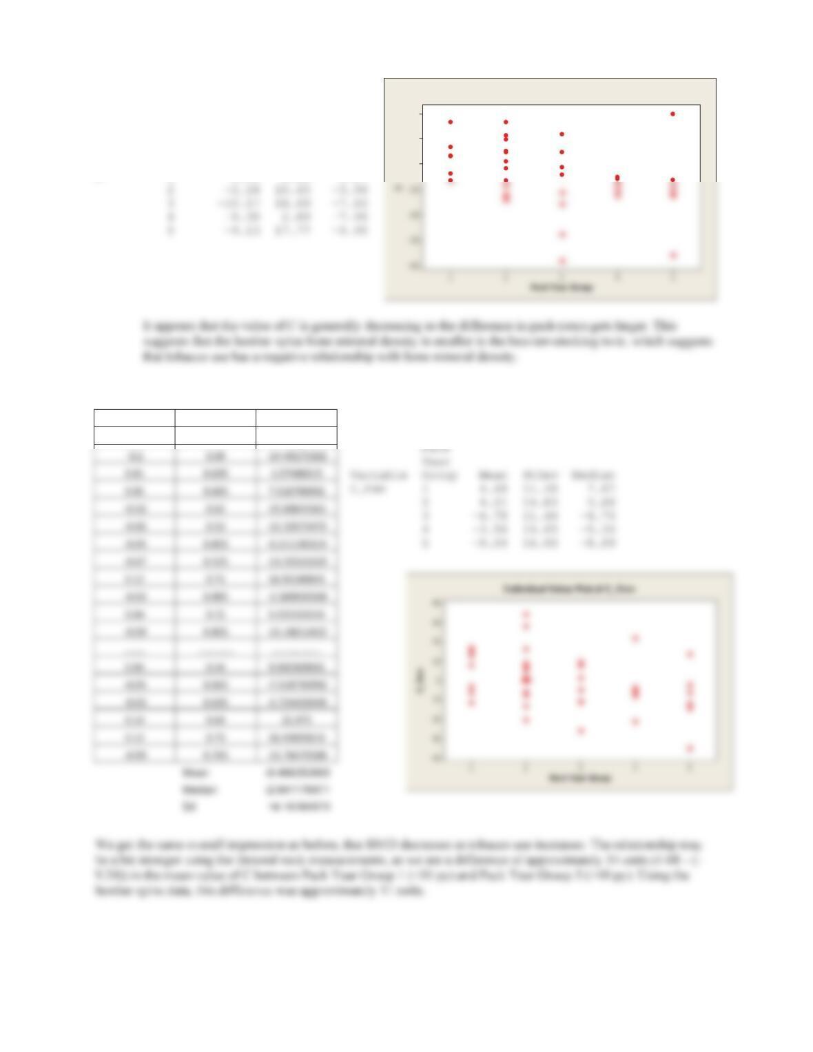
2.38-2.40 For lumbar spine bone mineral density, we have the following:

ID A B C PYDiffPackYearGroup

1002501 Ͳ0.050.785Ͳ6.3694267513.752

1015401 Ͳ0.120.95Ͳ12.6315789485

1027601 Ͳ0.240.63Ͳ38.095238120.53

1034301 0.040.834.8192771129.753

CHAPTER 2/DESCRIPTIVE STATISTICS 18

Descriptive Statistics: C

Pack

Year

Variable Group Mean StDev Median

C 1 1.95 8.26 3.17

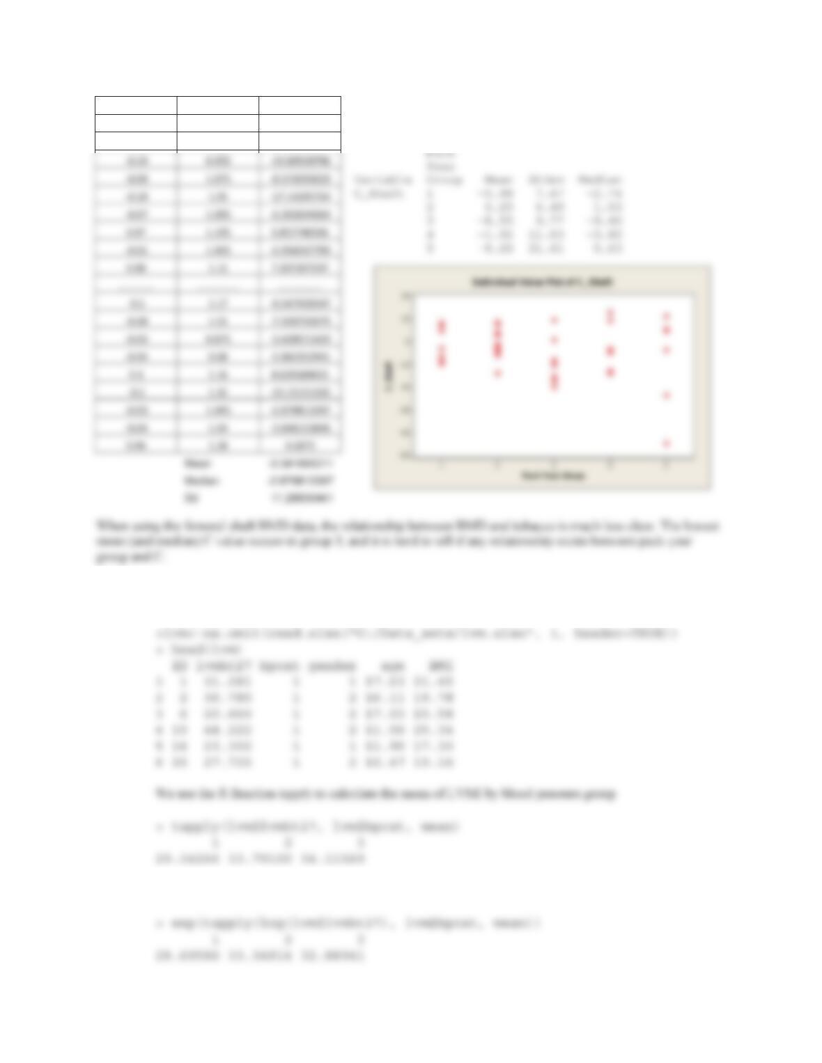
2.41-2.43 For femoral neck BMD, we find . . .

Descriptive Statistics: C_Fem

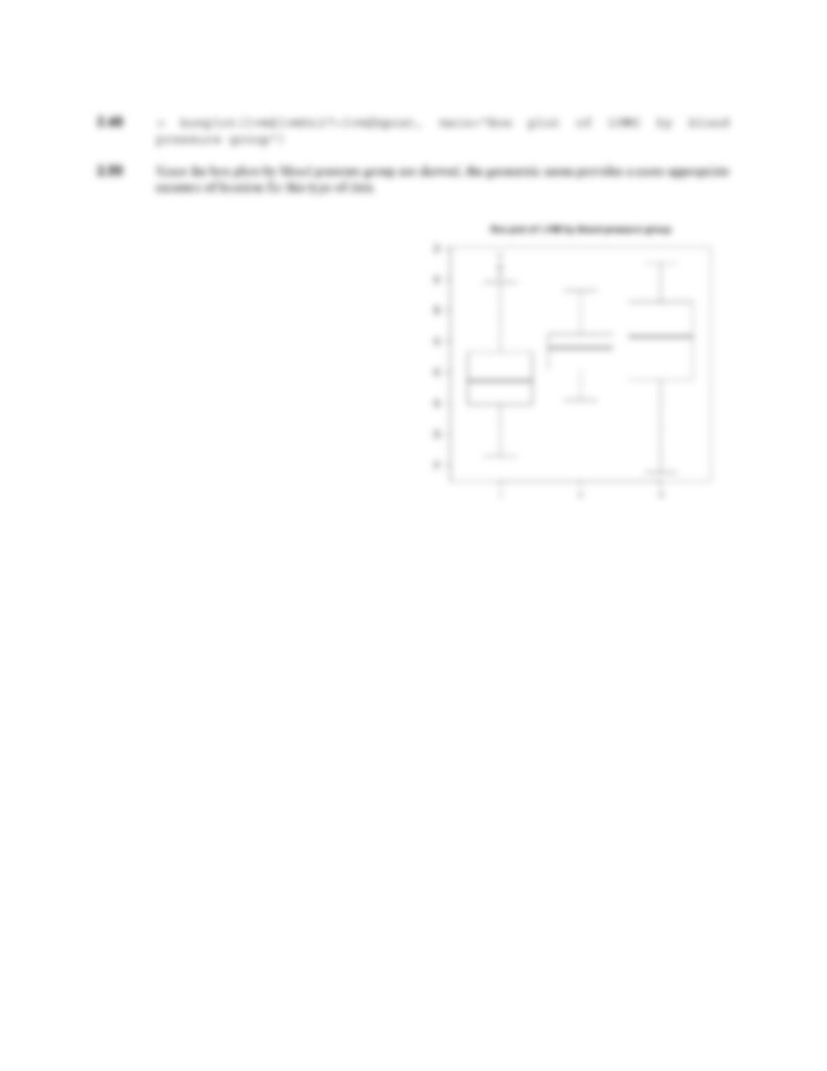
2.44-2.46 Using femoral shaft BMD, we find the following:

A B C

Ͳ0.040.7Ͳ5.714285714

20

10

0

Individual Value Plot of C

CHAPTER 2/DESCRIPTIVE STATISTICS 19

Descriptive Statistics: C_Shaft

2.47 We first read the data set LVM and show its first observations

> require(xlsx)

2.48 We use also the R function tapply to calculate the geometric mean of LVMI by blood pressure group

A B C

0.041.023.921568627

0.121.0511.42857143

CHAPTER 2/DESCRIPTIVE STATISTICS 20