Accounting Chapter 19 Homework Note The Asset Disposed The End The

19–17

Problem 19.24 (Concluded)

4. Most of the factors mentioned can be quantified. Furthermore, they should be

included in the analysis. All direct and indirect costs as well as costs of in-

tangible factors should be included; otherwise, it is possible to miss out on a

very profitable investment. The exclusion of the environmental fine is espe-

Annual cash flows increase by $135,000 (fines and sales effect) [e.g., cash

inflows increase to $340,200 in Year 1 ($205,200 + $135,000) and $358,200 for

Years 2–7 ($223,200 + $135,000)].

Payback:

Problem 19.25

1. Traditional equipment (18% rate):

Year Cash Flow df Present Value

3–10 ……………………………….. 200,000 2.928 585,600

NPV …………………………………………………………………………….. $ 381,000

19–18

Problem 19.25 (Continued)

Contemporary technology:

Year Cash Flow df Present Value

0 ………………………………….. $(4,000,000) 1.000 $(4,000,000)

2 ………………………………….. 400,000 0.718 287,200

3 ………………………………….. 600,000 0.609 365,400

4–6 ………………………………… 800,000 1.323 1,058,400

7 ………………………………….. 1,000,000 0.314 314,000

2. Traditional equipment (14% rate):

Year Cash Flow df Present Value

0 ………………………………….. $(1,000,000) 1.000 $(1,000,000)

1 ………………………………….. 600,000 0.877 526,200

Contemporary technology:

Year Cash Flow df Present Value

0 ………………………………….. $(4,000,000) 1.000 $(4,000,000)

1 ………………………………….. 200,000 0.877 175,400

7 ………………………………….. 1,000,000 0.400 400,000

3. The cost of capital is the rate that should be used—it usually reflects the op-

portunity cost of the funds needed to make the investment. A higher rate will

bias against the acceptance of contemporary technology—which usually has

19–19

Problem 19.25 (Concluded)

4. Traditional equipment:

Year Cash Flow df Present Value

0 ………………………………….. $(1,000,000) 1.000 $(1,000,000)

1 ………………………………….. 600,000 0.877 526,200

Problem 19.26

1. Scrubbers and treatment facility (expressed in thousands):

Present

Year (1 – t)Ra –(1 – t)Cb tNCc CF df Value

0 …….. $(50,000) 1.000 $(50,000)

1 …….. $6,000 $(14,400) $4,000 (4,400) 0.909 (4,000)

2 …….. 6,000 (14,400) 6,400 (2,000) 0.826 (1,652)

a0.6 × $10,000,000 = $6,000,000

b0.6 × $24,000,000 = $14,400,000

cYear 1: 0.4 × (0.2 × $50,000,000)

Year 2: 0.4 × (0.32 × $50,000,000)

19–20

Problem 19.26 (Concluded)

Process redesign (expressed in thousands):

Present

Year (1 – t)Ra –(1 – t)Cb tNCc CF df Value

0 …….. $(100,000) 1.000 $(100,000)

1 …….. $18,000 $(6,000) $ 8,000 20,000 0.909 18,180

2 …….. 18,000 (6,000) 12,800 24,800 0.826 20,485

a0.6 × $30,000,000 = $18,000,000

b0.6 × $10,000,000 = $6,000,000

cYear 1: 0.4 × (0.2 × $100,000,000)

2. The modification will add to the cost of the scrubbers and treatment facility

$30.04 and $45.06 million to the first (second) alternative (0.751 × $40,000,000)

and (0.751 × $60,000,000). Adding in the benefit of avoiding the cleanup cost

makes the process redesign alternative profitable (yielding a positive NPV).

Problem 19.27

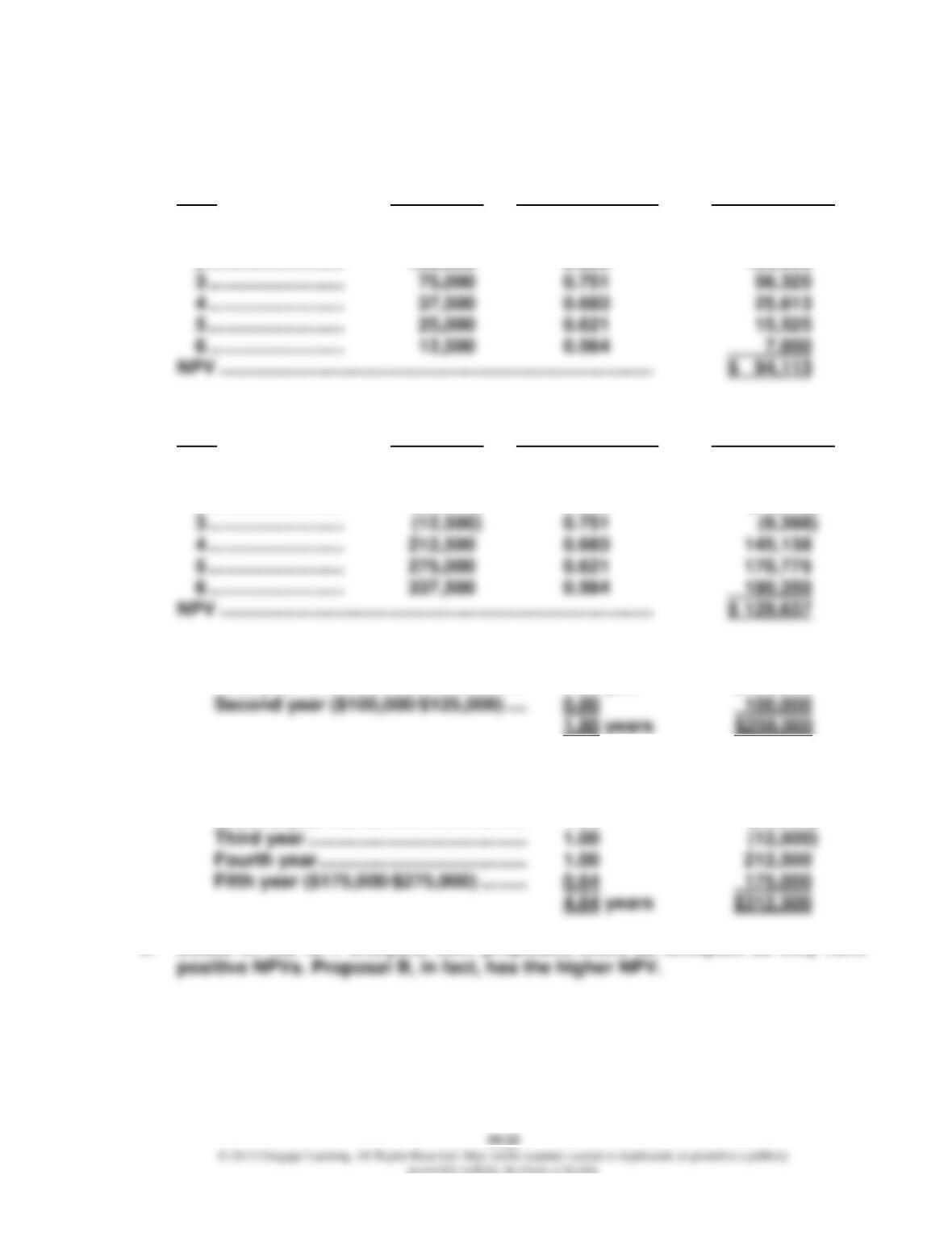
1. Proposal A:

Year Cash Flow Discount Factor Present Value

0 …………………….. $(250,000) 1.000 $(250,000)

1 …………………….. 150,000 0.909 136,350

2 …………………….. 125,000 0.826 103,250

Proposal B:

Year Cash Flow Discount Factor Present Value

0 …………………….. $(312,500) 1.000 $(312,500)

1 …………………….. (37,500) 0.909 (34,088)

2 …………………….. (25,000) 0.826 (20,650)

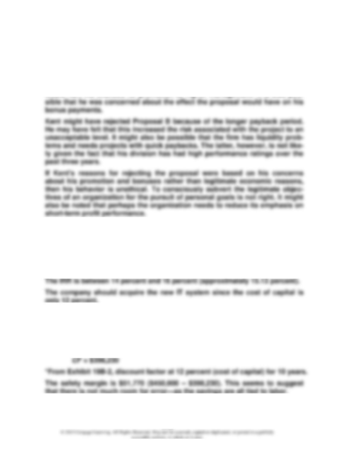
2. Proposal A payback period:

First year ……………………………………. 1.00 year $150,000

Proposal B payback period:

First year ……………………………………. 1.00 year $ (37,500)

Second year ……………………………….. 1.00 (25,000)

3. Based on the NPV analysis, both proposals could be accepted as they have

19–22

Problem 19.27 (Concluded)

4. Kent Tessman may have accepted only Proposal A because of the fact that

his performance is going to be closely monitored over the next three years.

Proposal B had negative cash flows projected for the first three years. This

would hurt his divisional profits during that time, and he may feel that this

would hurt his chances for promotion to higher management. It is also pos-

Problem 19.28

1. df = Investment/Annual cash flow

= $2,250,000/$450,000

= 5.0

2. Since I = P for the IRR, the minimum cash flow is:

I = df × CF

$2,250,000 = 5.650* × CF

5.650 × CF = $2,250,000

CF = $2,250,000/5.650

19–23

Problem 19.28 (Concluded)

3. For a life of eight years:

df = I/CF

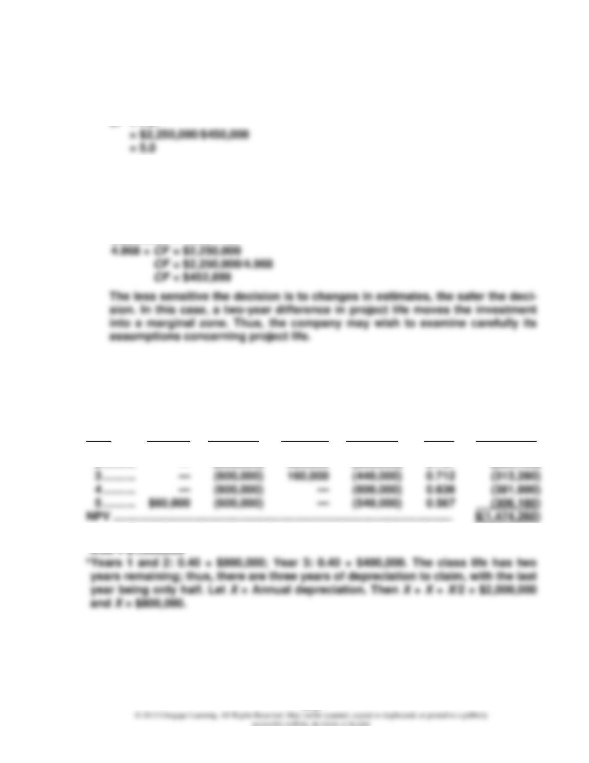
The IRR is between 10 percent and 12 percent (approximately 11.83 percent).

The system is about at the break-even point (point of indifference).

Minimum cash flow at 12 percent for eight years:

I = df × CF

$2,250,000 = 4.968 × CF

Problem 19.29

Keep old MRI equipment:

Present

Year (1 – t)Ra –(1 – t)Cb tNCc CF df Value

1 ………. — $(600,000) $320,000 $(280,000) 0.893 $ (250,040)

2 ………. — (600,000) 320,000 (280,000) 0.797 (223,160)

a0.60 × $100,000

b0.60 × $1,000,000

19–24

Problem 19.29 (Concluded)

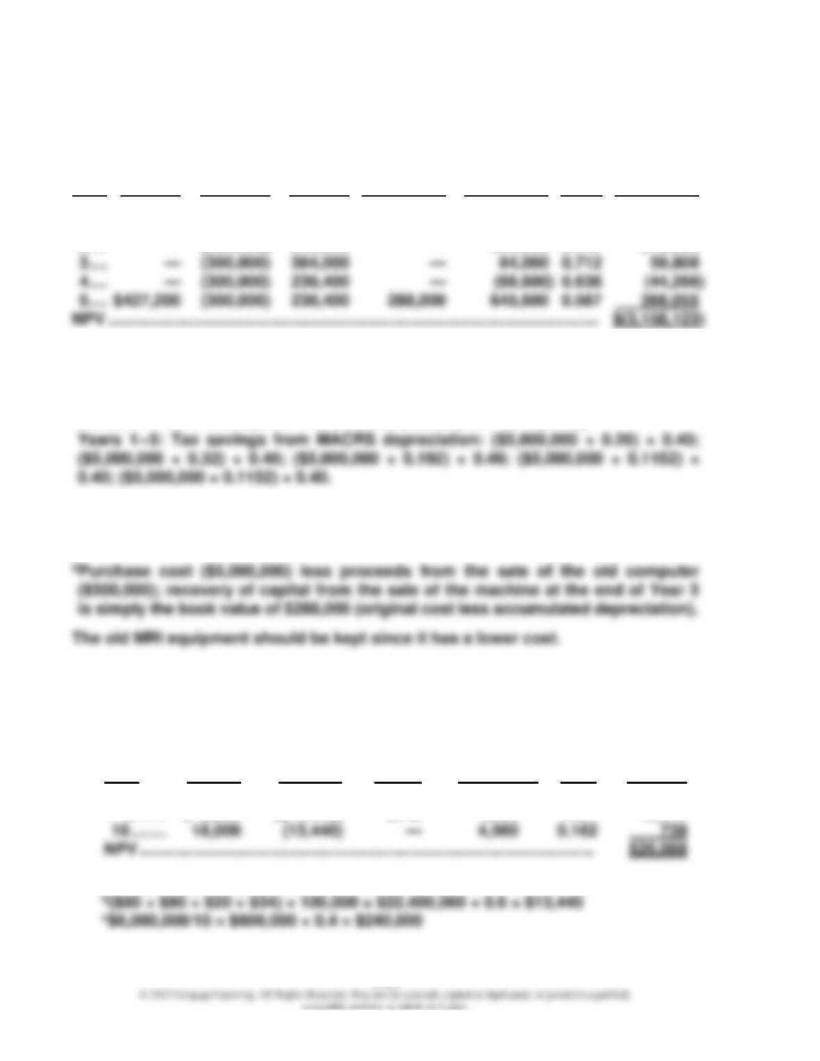
Buy new MRI equipment:

Present

Year (1 – t)Ra –(1 – t)Cb tNCc Otherd CF df Value

0 …. — $600,000 $(4,500,000) $(3,900,000) 1.000 $(3,900,000)

1 …. — $(300,000) 400,000 — 100,000 0.893 89,300

2 …. — (300,000) 640,000 — 340,000 0.797 270,980

a0.60 × ($1,000,000 – Book value), where Book value = $5,000,000 – $4,712,000.

b0.60 × $500,000.

cYear 0: Tax savings from loss on sale of asset: 0.40 × $1,500,000 [(The loss on

the sale of the old computer is $1,500,000 ($2,000,000 – $500,000.)]

Note: The asset is disposed of at the end of the fifth year—the end of its class

life—so the asset is held for its entire class life, and the full amount of deprecia-

tion can be claimed in Year 5.

Problem 19.30

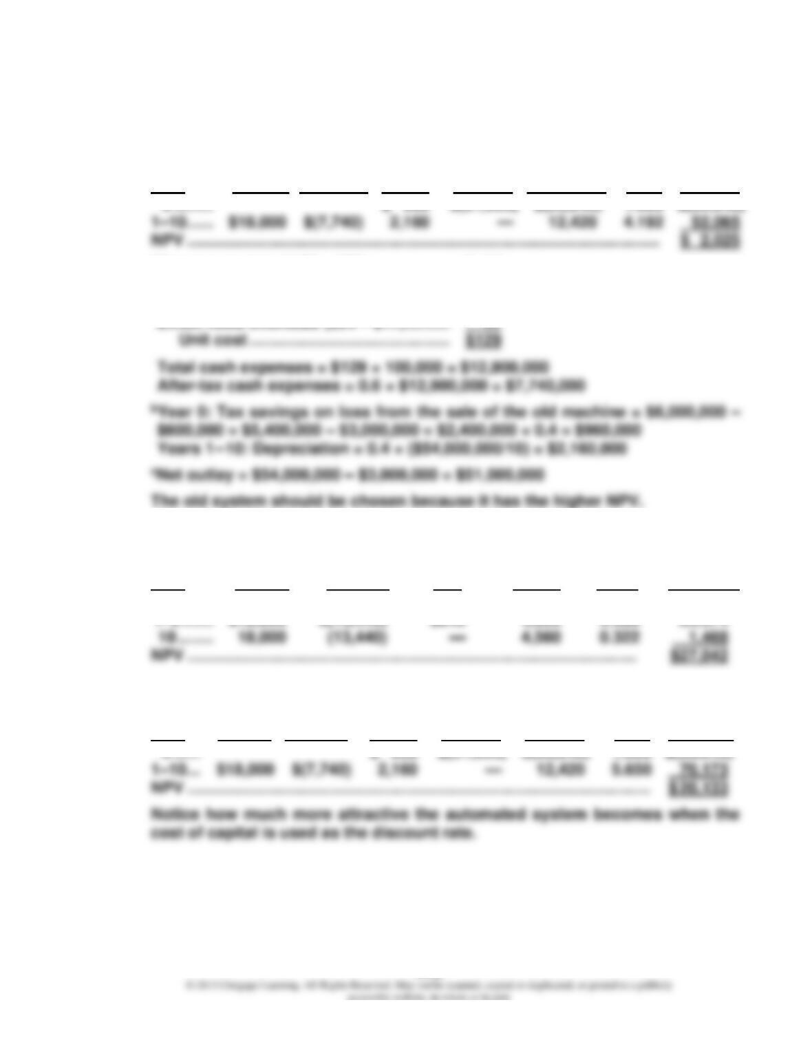
1. Old system (dollars in thousands):

Present

Year (1 – t)Ra –(1 – t)Cb tNCc Cash Flow df Value

0 ……… $ 0 1.000 $ 0

1–9 ……. $18,000 $(13,440) $240 4,800 4.031 19,349

a100,000 × $300 = $30,000,000 × 0.6 = $18,000,000

19–25

Problem 19.30 (Continued)

New system (dollars in thousands):

Present

Year (1 – t)R –(1 – t)Ca tNCb Otherc Cash Flow df Value

0 ……… $ 960 $(51,000) $(50,040) 1.000 $(50,040)

aDirect materials (0.75 × $80) ……………… $ 60

Direct labor (0.4 × $90) ……………………… 36

Volume-related overhead ($20 – $4) ….. 16

Direct fixed overhead ($34 – $17) ………. 17

2. Old system (dollars in thousands):

Present

Year (1 – t)R –(1 – t)C tNC CF df Value

0 ……… $ 0 1.000 $ 0

1–9 ……. $18,000 $(13,440) $240 4,800 5.328 25,574

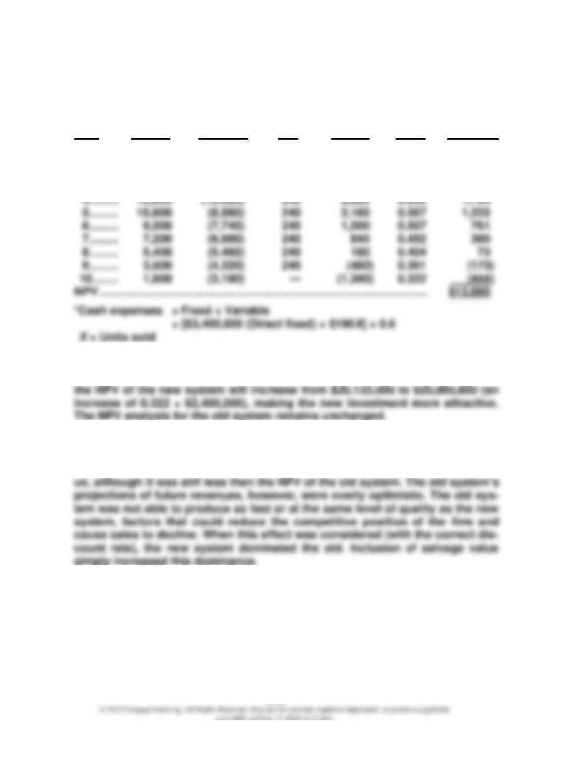
New system (dollars in thousands):

Present

Year (1 – t)R –(1 – t)C tNC Other CF df Value

0 …… $ 960 $(51,000) $(50,040) 1.000 $(50,040)

19–26

Problem 19.30 (Concluded)

3. Old system with declining sales (dollars in thousands):

Present

Year (1 – t)R –(1 – t)C* tNC CF df Value

0 ……… $ 0 1.000 $ 0

1 ……… $18,000 $(13,440) $240 4,800 0.893 4,286

2 ……… 16,200 (12,300) 240 4,140 0.797 3,300

3 ……… 14,400 (11,160) 240 3,480 0.712 2,478

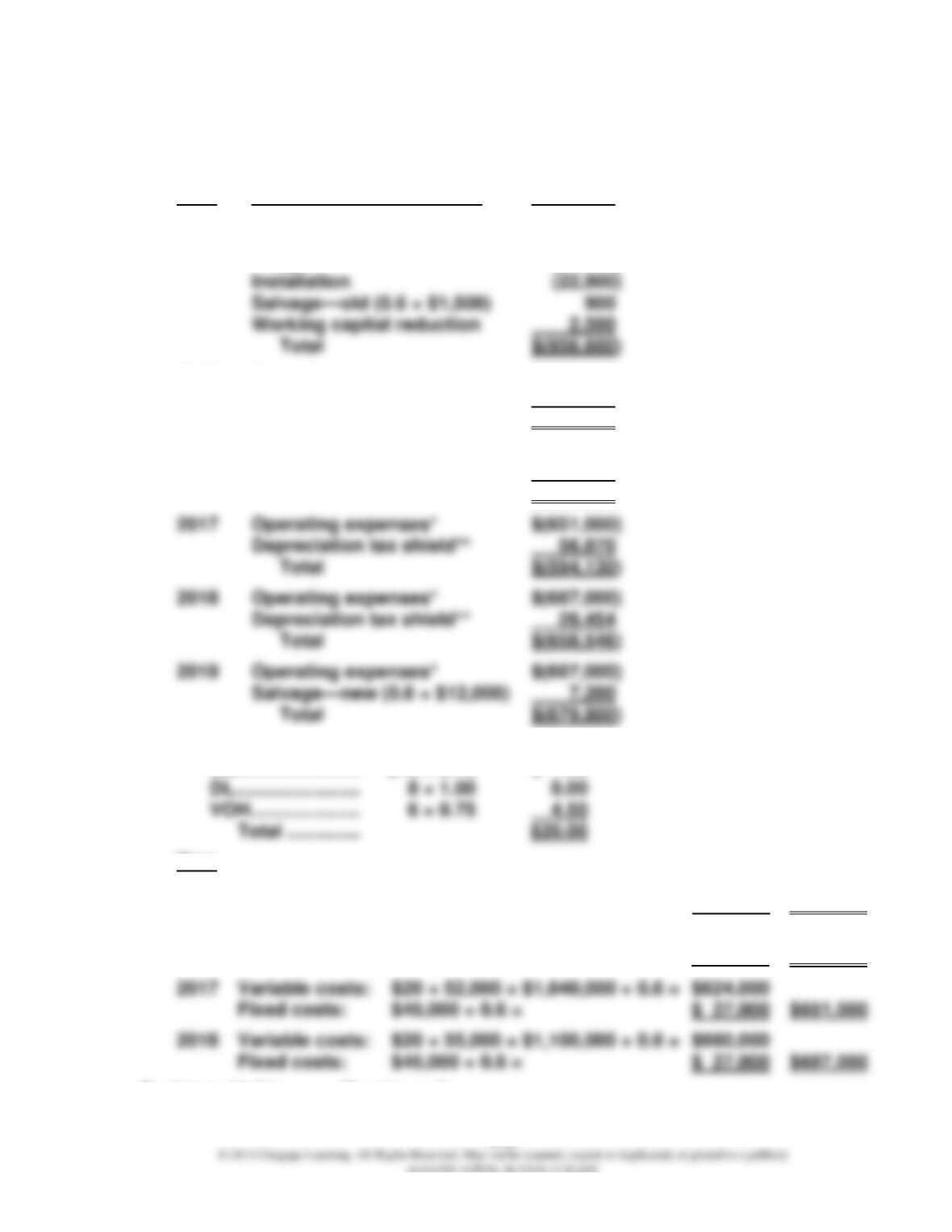
4. For the new system, salvage value would increase after-tax cash flows in

Year 10 by $2,400,000 (0.6 × $4,000,000). Using the discount factor of 0.322,

5. Requirement 2 illustrates the importance of using the correct discount rate.

The rate of 20 percent made the automated alternative look totally unappeal-

ing. By using the correct rate, the alternative showed a large net present val-

19–27

Problem 19.31

1. Schedule of cash flows:

Year Item CF

2014 Equipment $(945,000)

Discount 18,900

Freight (11,000)

2015 Operating expenses* $(627,000)

Depreciation tax shield** 127,987

Total $(499,013)

2016 Operating expenses* $(627,000)

Depreciation tax shield** 170,688

Total $(456,312)

*Unit cost:

DM ………………….. $10 × 0.75 $ 7.50

Year

2015 Variable costs: $20 × 50,000 = $1,000,000 × 0.6 = $600,000

Fixed costs: $45,000 × 0.6 = $ 27,000 $627,000

2016 Variable costs: $20 × 50,000 = $1,000,000 × 0.6 = $600,000

Fixed costs: $45,000 × 0.6 = $ 27,000 $627,000

Problem 19.31 (Continued)

19–28

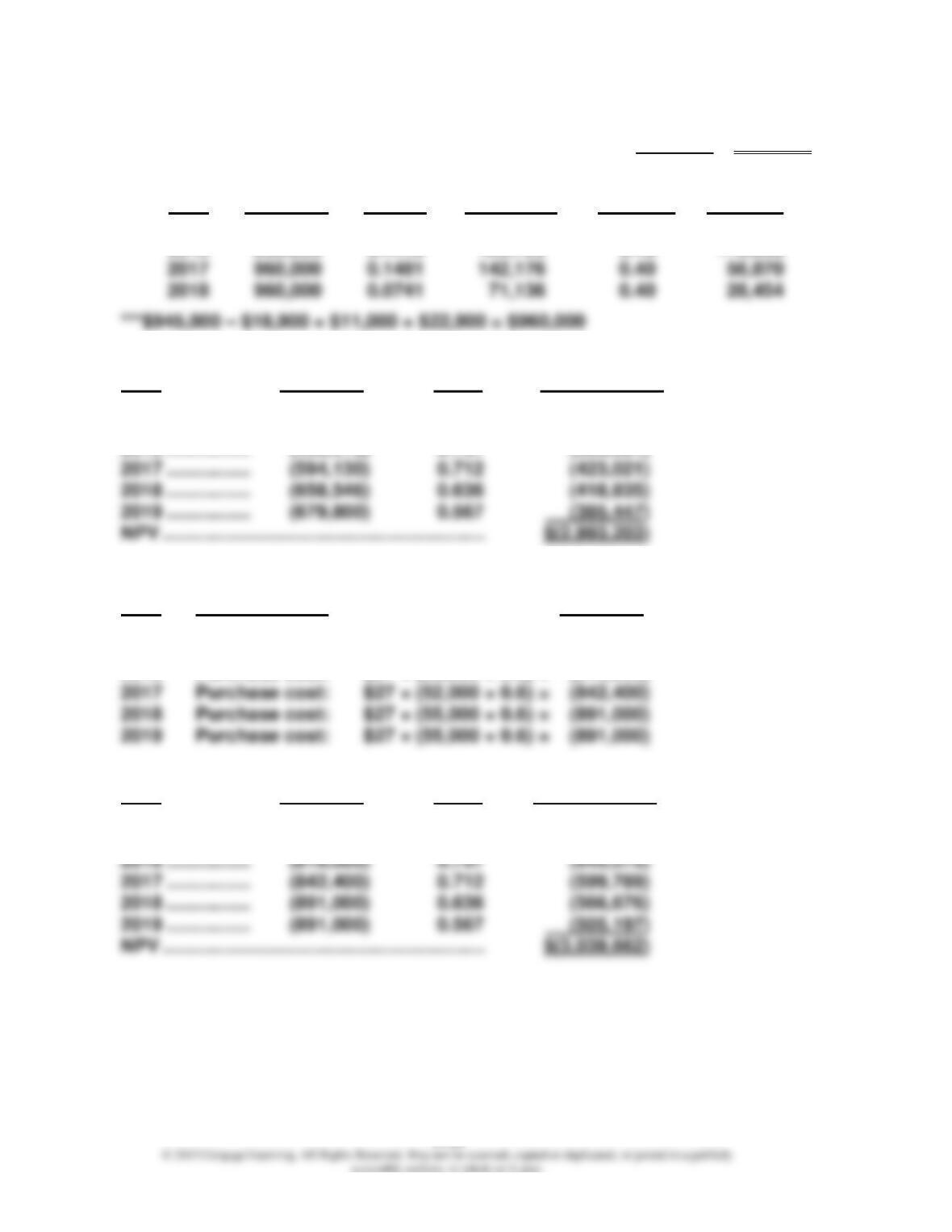
2019 Variable costs: $20 × 55,000 = $1,100,000 × 0.6 = $660,000

Fixed costs: $45,000 × 0.6 = $ 27,000 $687,000

**Depreciation tax shield:

Year Value*** Rate Allowance Tax Rate Shield

2015 $960,000 0.3333 $319,968 0.40 $127,987

2016 960,000 0.4445 426,720 0.40 170,688

NPV:

Year CF df Present Value

2014 ……………. $(956,600) 1.000 $ (956,600)

2015 ……………. (499,013) 0.893 (445,619)

2016 ……………. (456,312) 0.797 (363,681)

2. Schedule of cash flows:

Year Item CF

2014 Salvage—old (0.6 × $1,500) = $ 900

2015 Purchase cost: $27 × (50,000 × 0.6) = (810,000)

2016 Purchase cost: $27 × (50,000 × 0.6) = (810,000)

NPV:

Year CF df Present Value

2014 ……………. $ 900 1.000 $ 900

2015 ……………. (810,000) 0.893 (723,330)

19–29

Problem 19.31 (Concluded)

3. The analysis favors internal production because it has a lower cost than pur-

Problem 19.32

1. After-tax cash flows:

Manual system:

Year (1 – t)Ra –(1 – t)Cb tNCc Cash Flows

a0.60 × $400,000 (sales)

Robotic system:

Year (1 – t)Ra –(1 – t)Cb tNCc Otherd Cash Flows

0 ….. $64,000 $(480,000) $(416,000)

1 ….. $240,000 $(124,320) 29,723 — 145,403

2 ….. 270,000 (132,960) 50,939 — 187,979

3 ….. 300,000 (141,600) 36,379 — 194,779

aYear 1: 0.60 × $400,000; Year 2: 0.60 × $450,000; Year 3: 0.60 × $500,000;

bAfter-tax cash expenses:

Fixed:

Direct labor …….. $20,000 × 0.60 = $12,000 (one operator)

19–30

Problem 19.32 (Continued)

Variable:

Direct materials ……. (0.16 × Sales) × 0.75 × 0.60 = 0.0720 × Sales

Variable overhead … (0.09 × Sales) × 0.6667 × 0.60 = 0.0360 × Sales

cYear 0: Tax savings on loss: [($200,000 – $40,000) × 0.40]

Years 1–8: MACRS: 0.1429 × ($520,000 × 0.40) 0.2449 × ($520,000 × 0.40) etc.

dNet investment:

Purchase costs …………………… $520,000

2. Manual system:

Year Cash Flow Discount Factor Present Value

0 ………….. $ 0 1.000 $ 0

Robotic system:

Year Cash Flow Discount Factor Present Value

0 ………….. $(416,000) 1.000 $(416,000)

1 ………….. 145,403 0.893 129,845

2 ………….. 187,979 0.797 149,819

3 ………….. 194,779 0.712 138,683

19–31

Problem 19.32 (Concluded)

3. Managers may use a higher discount rate as a way to deal with the uncertain-

ty in future cash flows. The higher rate “protects” the manager from

unpleasant surprises. Since a higher rate favors investments that provide

returns quickly, managers may be motivated by personal short-run consider-

ations (e.g., bonuses and promotion opportunities).

Using a discount rate of 12%:

Year Cash Flow Discount Factor Present Value

0 ………….. $(340,000) 1.000 $(340,000)

1–10 ……….. 80,000 5.650 452,000

NPV ………………………………………………………… $ 112,000

1–10 ……….. 80,000 4.192 335,360

NPV ………………………………………………………… $ (4,640)

If the 20 percent discount rate is used, the company would not acquire the

robotic system.

CYBER RESEARCH CASE

19.33

Answers will vary.

The Collaborative Learning Exercise Solutions can be found on the

19–32

The following problems can be assigned within CengageNOW and are auto-

graded. See the last page of each chapter for descriptions of these new assign-

ments.

• Integrative Exercise—CVP, Break-Even Analysis, Theory of Constraints (Co-

vers chapters 16, 19, and 20)