18–19
PROBLEMS
Problem 18.26
Chain store costs: Small retail store costs:
Sales salaries …………. $ 110,000 Sales support ……………… $ 328,000
Delivery cost* …………. 51,000 Delivery cost** …………….. 142,800
Problem 18.27
1. Total Cost Per Unit
Direct materials ………………. $ 540,000 $ 6.00
Direct labor …………………….. 99,000 1.10
2. Total Cost Per Unit
Direct materials ………………. $ 540,000 $ 6.00
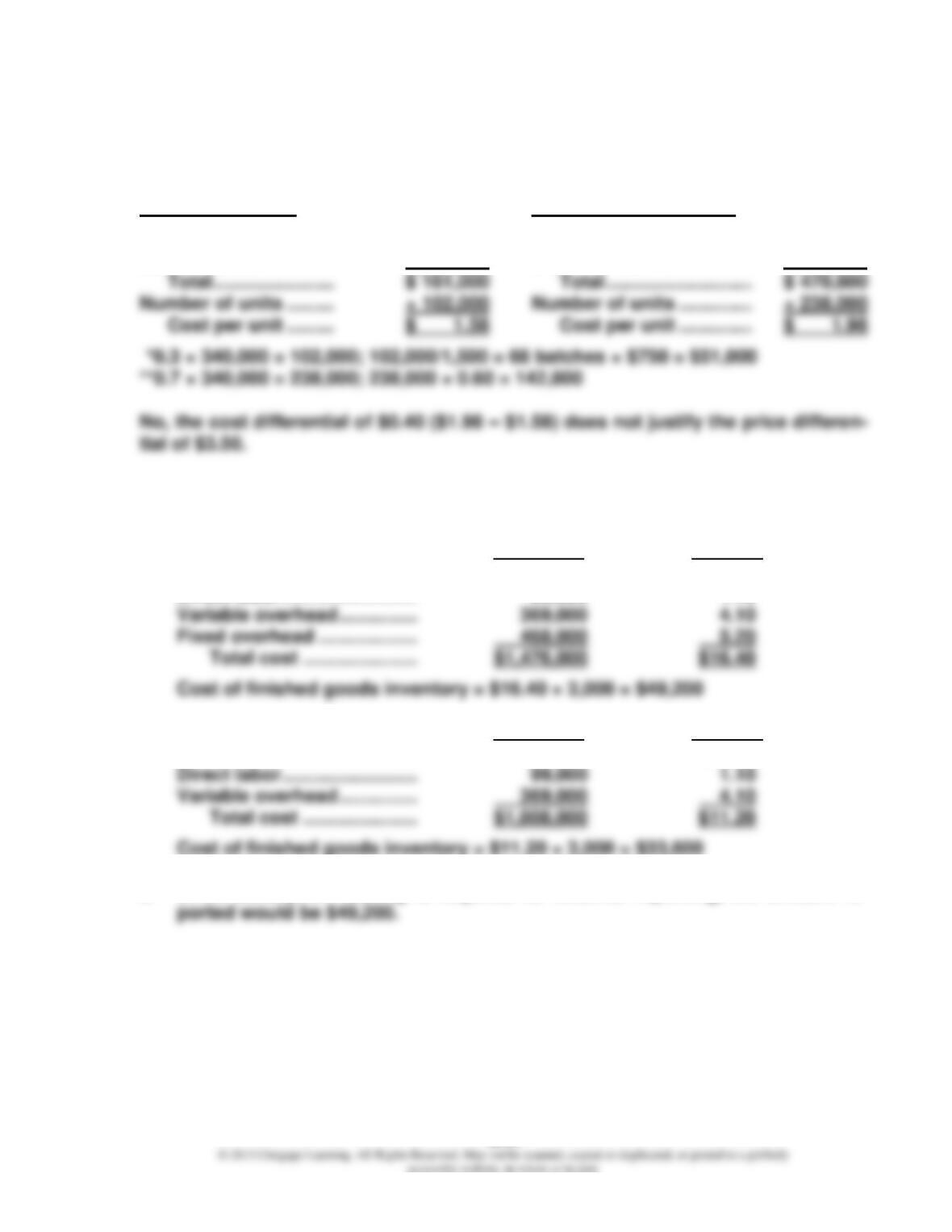
3. Since absorption costing is required for external reporting, the amount re-
18–20
Problem 18.28
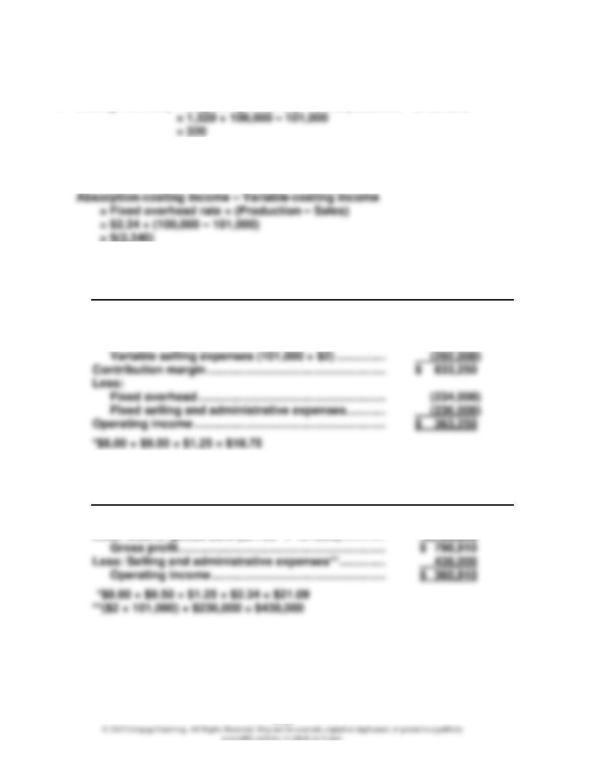
1. Ending inventory = Beginning inventory + Units produced – Units sold
2. Fixed overhead rate = $234,000/100,000 = $2.34 per unit
The difference is given as follows:
3. a. Vladamir, Inc.
Variable-Costing Income Statement
For Last Year
Sales ($29 × 101,000) …………………………………………….. $ 2,929,000
Less:
Variable cost of goods sold (101,000 × $18.75*) …. (1,893,750)
b. Vladamir, Inc.
Absorption-Costing Income Statement
For Last Year
Sales ($29 × 101,000) …………………………………………….. $2,929,000
Less: Cost of goods sold ($21.09* × 101,000) …………. 2,130,090
18–21
Problem 18.29
1. Jellison Company
Absorption-Costing Income Statement
For Years 1 and 2
Year 1 Year 2
Sales ……………………………………………………………………. $960,000 $1,080,000
Less: Cost of goods solda ……………………………………… 832,000 956,000
Gross profit ……………………………………………………… $128,000 $124,000
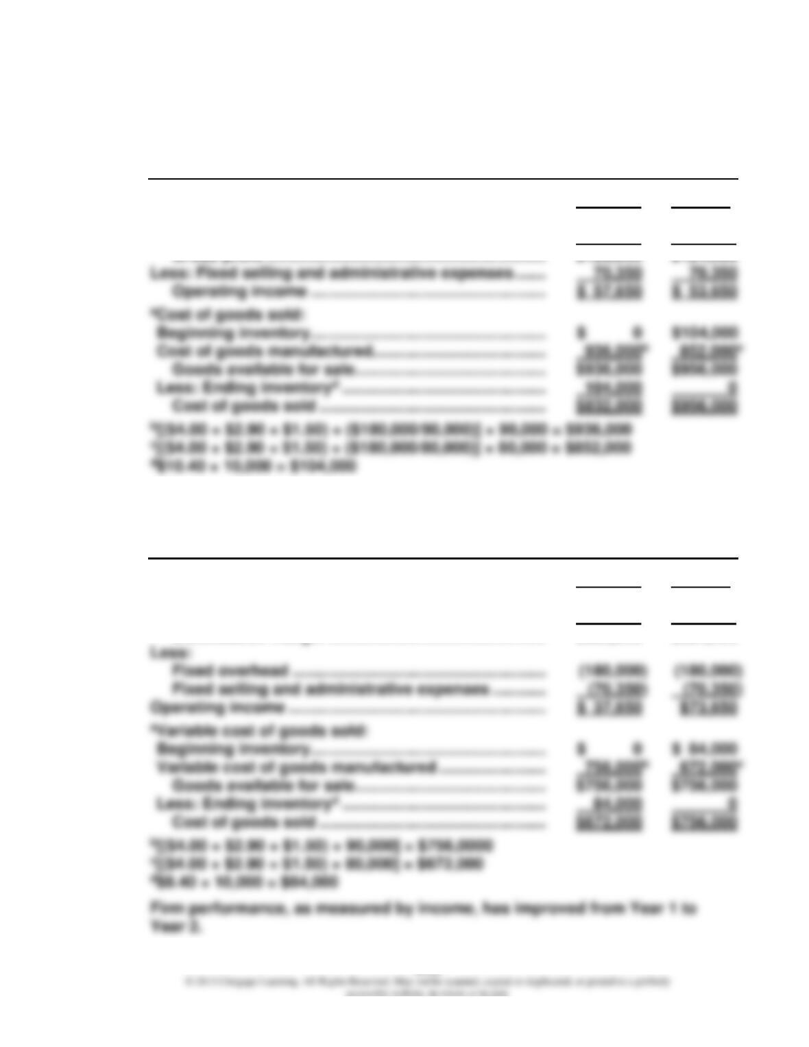
Firm performance, as measured by income, has improved from Year 1 to Year 2.
2. Jellison Company
Variable-Costing Income Statement
For Years 1 and 2
Year 1 Year 2
Sales ……………………………………………………………………. $960,000 $1,080,000
Less: Variable cost of goods solda ………………………… 672,000 756,000
Contribution margin …………………………………………. $288,000 $324,000
18–22
Problem 18.29 (Concluded)
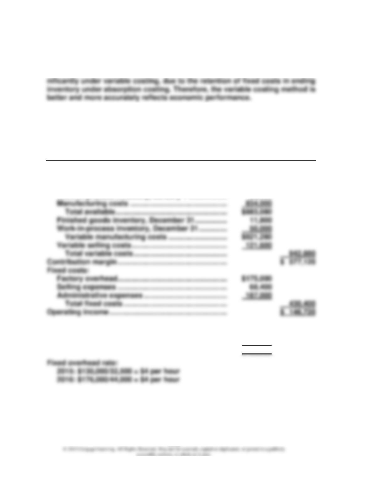
3. Since sales have increased with costs remaining the same, one would expect
an increase in income. Income increases under both methods, but more sig-
Problem 18.30
1. San Mateo Optics, Inc.
Variable-Costing Income Statement
For the Year Ended December 31, 2016
Net sales ………………………………………………………………. $1,520,000
Variable costs:
Finished goods inventory, January 1 ………………… $ 20,680
Work-in-process inventory, January 1 ………………. 28,400
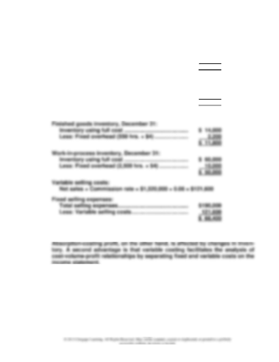
Finished goods inventory, January 1:
Inventory using full cost …………………………………… $ 25,000
Less: Fixed overhead (1,080 hrs. × $4) ………………. 4,320
$ 20,680
18–23
Problem 18.30 (Concluded)
Work-in-process inventory, January 1:
Inventory using full cost …………………………………… $ 34,000
Less: Fixed overhead (1,400 hrs. × $4) ………………. 5,600
$ 28,400
Manufacturing costs:
Direct materials ………………………………………………… $210,000
Direct labor ………………………………………………………. 435,000
Variable overhead (42,000 hrs. × $4.50) ……………… 189,000
$834,000
Variable overhead rate = $198,000/44,000 = $4.50 per hour
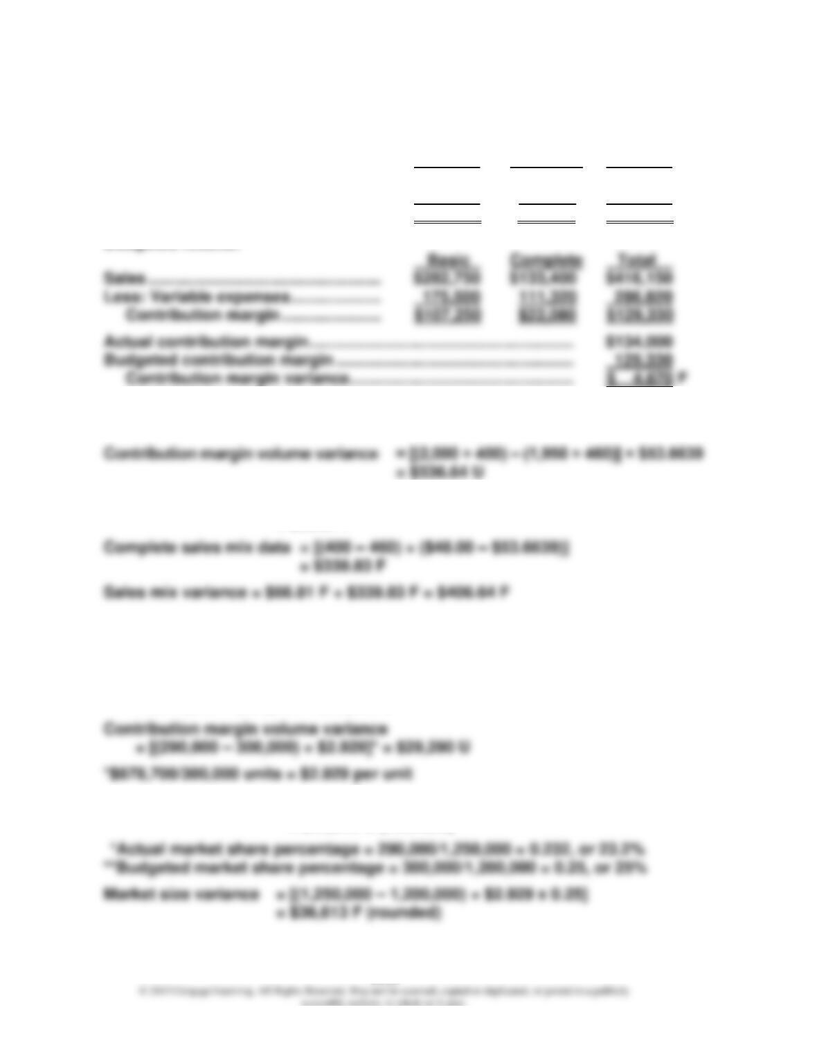
2. One advantage is that variable-costing financial statements are more easily
understood, since they show that profits move in the same direction as sales.
18–24
Problem 18.31
1. Actual results:
Basic Complete Total
Sales ……………………………………………. $280,000 $120,000 $400,000
Less: Variable expenses ……………….. 170,000 96,000 226,000
Contribution margin …………………. $110,000 $24,000 $134,000
Budgeted results:
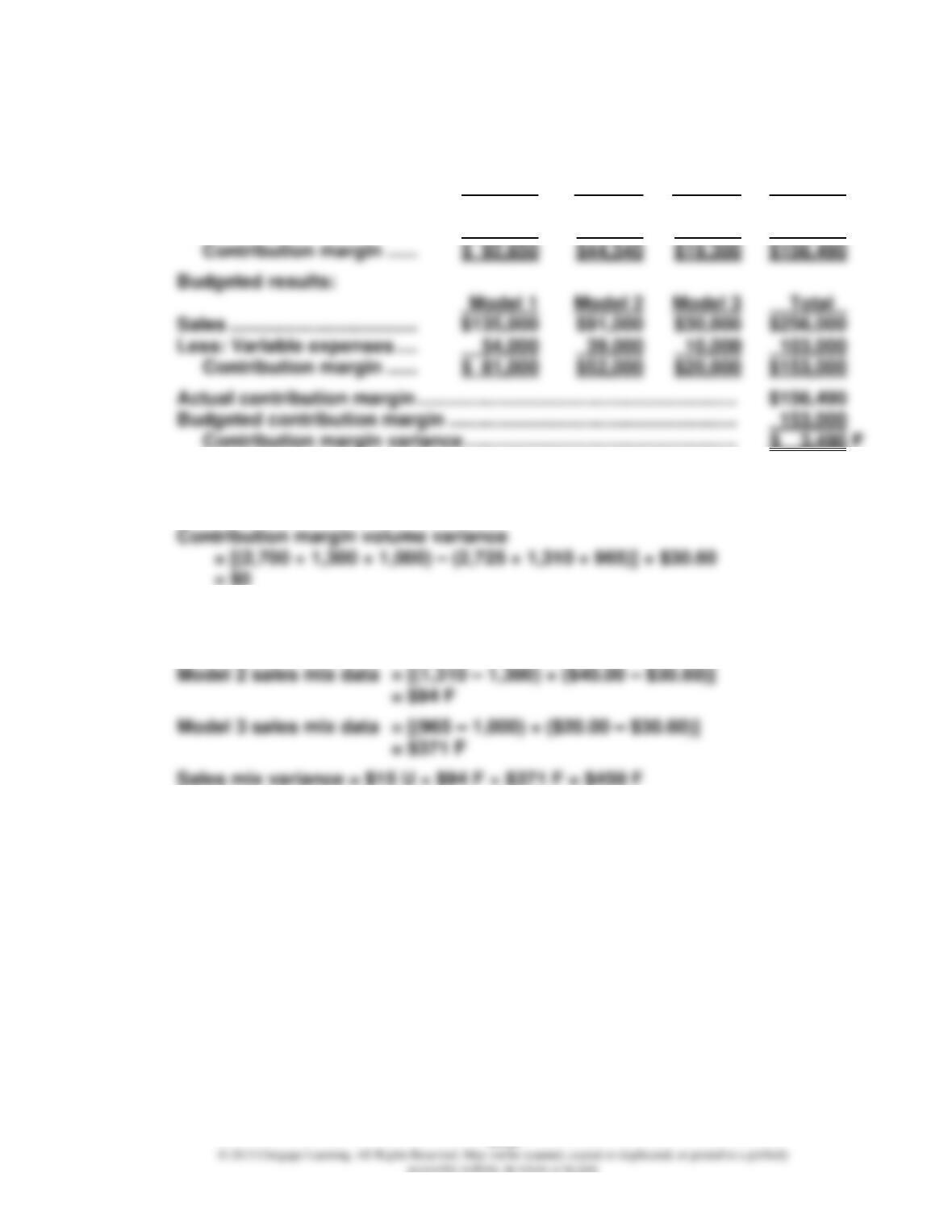
2. Budgeted average unit contribution margin = $129,330/2,410
= $53.6639
3. Basic sales mix data = [(2,000 – 1,950) × ($55.00 – $53.6639)]
= $66.81 F
Problem 18.32
1. Contribution margin variance
= $797,500 – $878,700 = $81,200 U
2. Market share variance = [(0.232* – 0.25**) × (1,250,000 × $2.929)]
= $65,903 U (rounded)
18–25
Problem 18.33
1. Actual results:
Model 1 Model 2 Model 3 Total
Sales ……………………………… $141,700 $89,080 $32,810 $263,590
Less: Variable expenses …. 49,050 44,540 13,510 107,100
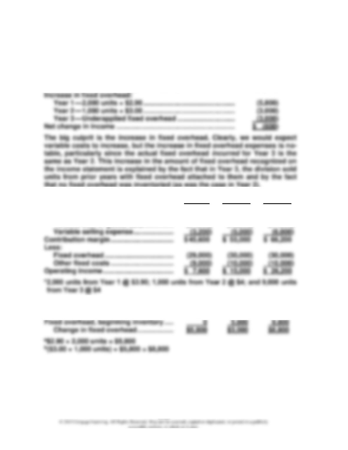
2. Budgeted average unit contribution margin = $153,000/5,000
= $30.60
3. Model 1 sales mix data = [(2,725 – 2,700) × ($30.00 – $30.60)]
= $15 U
18–26
Problem 18.34
1. The profit change can be explained by the following analysis:
Increase in sales revenue ……………………………………………….. $20,000
Increase in variable manufacturing costs ($3.90 × 2,000) ….. (7,800)
Increase in variable selling ($0.50 × 2,000)……………………….. (1,000)
2. Year 1 Year 2 Year 3
Sales …………………………………………………. $ 80,000 $100,000 $120,000
Less:
Variable cost of goods sold ……………. (31,200) (40,000) (47,800)*
Reconciliation:
Fixed overhead, ending inventory ………. $5,800a $8,800b $ 0
18–27
Problem 18.34 (Concluded)
The difference in the two income figures (absorption vs. variable) is exactly
explained by the change in fixed overhead in the division’s inventories. In
Year 1, $5,800 of the period’s fixed overhead was inventoried, thus explaining
why absorption-costing income was greater than variable costing by $5,800.
3. Since variable-costing income would have provided an increase in income
when sales increased (with no change in the costs of the period), the
Problem 18.35
1. There are many legitimate reasons that support the creation of inventory
(e.g., the need to avoid stockouts and the need to insure on-time delivery).
2. Since the decision to produce for inventory was not motivated by any sound
economic reasoning, and Bill knows the real motive behind the decision, he
should feel discomfort in the role he has been asked to assume. If he decides
to appeal to higher-level management, the divisional manager can counter
18–28
Problem 18.35 (Concluded)
3. The following standards may apply:
Competence—Provide decision support information and recommendations
that are accurate, clear, concise, and timely.
Problem 18.36
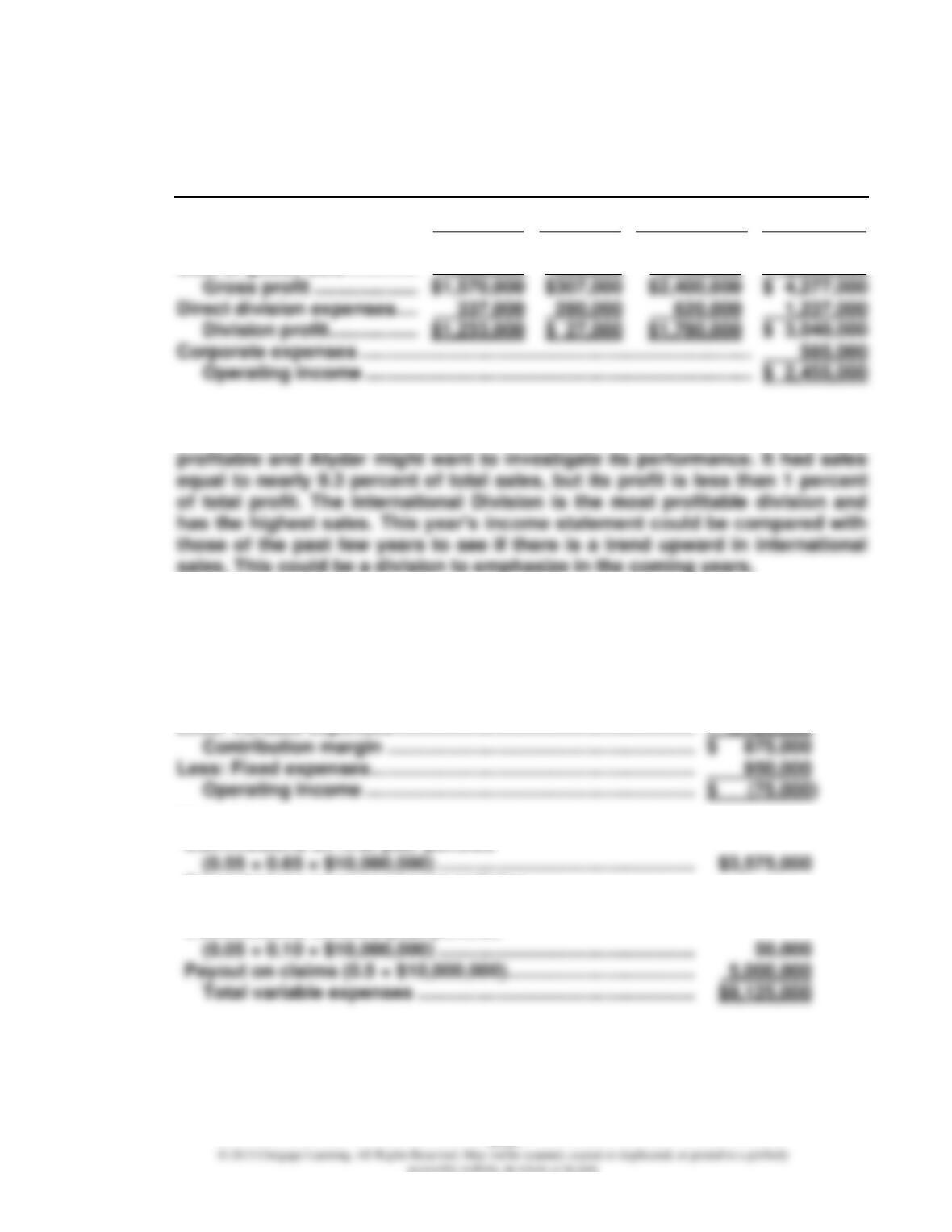
1. Products (in thousands)
A B C Total
Sales …………………………………….. $1,800 $1,740.0 $700.00 $4,240.00
2. Products (in thousands)
A D Total
Sales ………………………………………. $1,800 $1,160 $2,960
Less: Variable expenses ………….. 1,200 435 1,635
18–29
Problem 18.37
1. Alydar, Inc.
Income Statement
Eastern Southern International Total
Sales ……………………………… $3,150,000 $987,000 $6,500,000 $10,637,000
Cost of goods sold …………. 1,580,000 680,000 4,100,000 6,360,000
2. On the basis of division profit, the International Division had the best perfor-
mance, followed by the Eastern Division. The Southern Division is barely
Problem 18.38
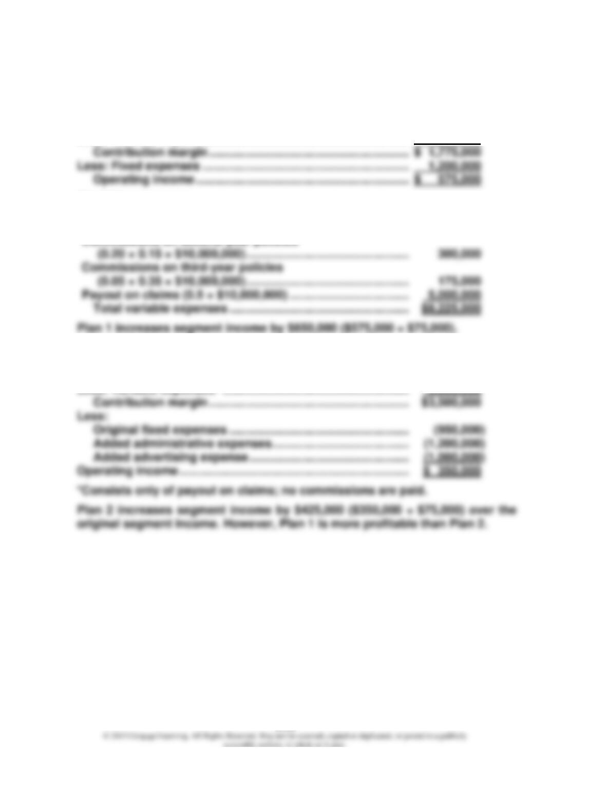
1. Operating income:
Sales …………………………………………………………………………….. $10,000,000
Less: Variable expenses ………………………………………………… 9,125,000*
*Variable expenses:
Commissions on first-year policies
Commissions on second-year policies
(0.20 × 0.25 × $10,000,000) …………………………………………. 500,000
Commissions on third-year policies
18–30
Problem 18.38 (Concluded)
2. Plan 1:
Sales ……………………………………………………………………………… $10,000,000
Less: Variable expenses …………………………………………………. 8,225,000*
*Variable expenses:
Commissions on first-year policies
(0.55 × 0.50 × $10,000,000) …………………………………………. $2,750,000
Commissions on second-year policies
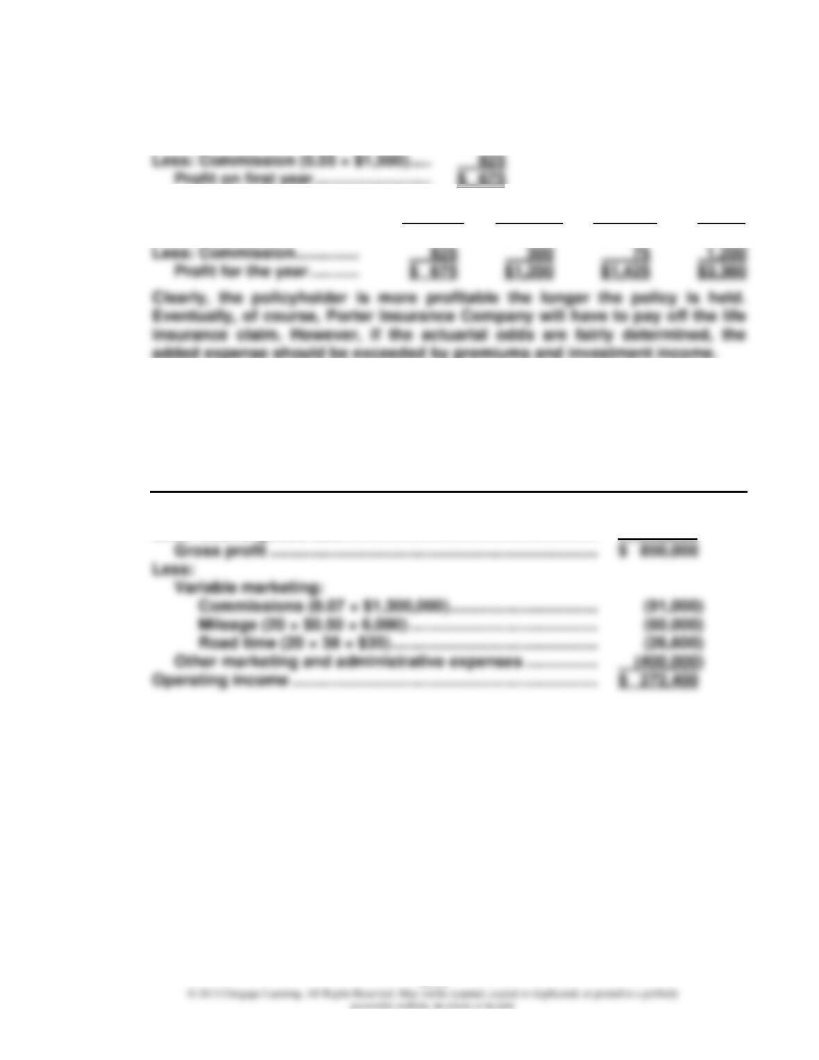
3. Plan 2:
Sales ……………………………………………………………………………… $7,000,000
Less: Variable expenses* ……………………………………………….. 3,500,000
18–31
Problem 18.39
1. Premium ………………………………………. $1,500
2. 1st Year 2nd Year 3rd Year Total
Premium ………………………… $1,500 $1,500 $1,500 $4,500
Problem 18.40
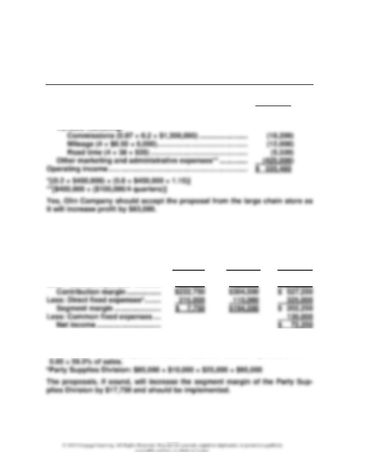
1. Olin Company
Income Statement
For the Coming Quarter
Sales …………………………………………………………………………….. $1,300,000
Less: Cost of goods sold ……………………………………………….. 450,000
18–32
Problem 18.40 (Concluded)
2. Olin Company
Revised Income Statement
For the Coming Quarter
Sales ……………………………………………………………………………… $1,300,000
Less: Cost of goods sold* ………………………………………………. 504,000
Gross profit ……………………………………………………………….. $ 796,000
Less:
Problem 18.41
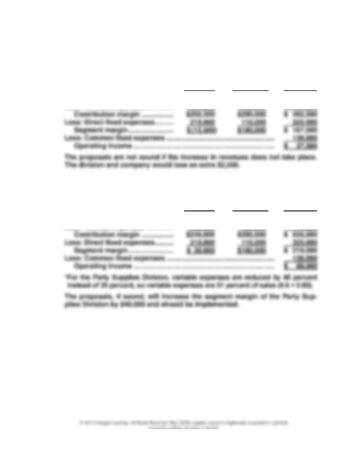
1. Party
Supplies Cookware
Division Division Total
Salesa ………………………………………. $550,000 $787,500 $1,337,500
Less: Variable expensesb …………. 327,250 483,000 810,250
aParty supplies sales: $500,000 × 1.10; Cookware sales: $750,000 × 1.05
bVariable expenses for the Party Supplies Division were $425,000/$500,000 =
85%. Under Paula’s proposal, variable costs are reduced by 30%, or 0.7 ×
18–33
Problem 18.41 (Concluded)
2. Paula’s proposals without increased sales:
Party
Supplies Cookware
Division Division Total
Sales ……………………………………….. $500,000 $750,000 $1,250,000
Less: Variable expenses …………… 297,500 460,000 757,500
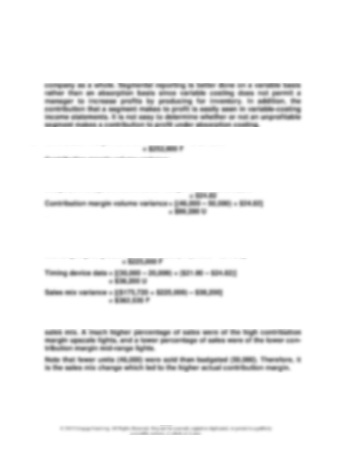
Paula’s proposals without increased sales but with 40 percent decrease in
variable costs:
Party
Supplies Cookware
Division Division Total
Sales ……………………………………….. $500,000 $750,000 $1,250,000
Less: Variable expenses* ………….. 255,000 460,000 715,000
18–34
Problem 18.42
1. An organization realizes a number of benefits from segmental reporting. In
particular, segmental reporting spotlights the profitability of each segment. In
this way, unprofitable segments are not lost in the overall profit of the
2. Contribution margin variance = $1,493,000 – $1,241,000
Contribution margin volume variance:
Actual units sold = 12,000 + 4,000 + 30,000 = 46,000
Budgeted units sales = 8,000 + 22,000 + 20,000 = 50,000
Budgeted average unit contribution margin = $1,241,000/50,000
Sales mix variance:
Upscale lighting data = (12,000 – 8,000)($68.75 – $24.82)
= $175,720 F
Mid-range lighting data = [(4,000 – 22,000) × ($12.32 – $24.82)]
3. The contribution margin variance is favorable because actual contribution
margin is higher than budgeted. This occurred because of the change in
18–35
18.43
Answers will vary.
The following problems can be assigned within CengageNOW and are auto-
graded. See the last page of each chapter for descriptions of these new assign-
ments.
• Analyzing Relationships—Vary actual (budgeted) prices and amounts to show
Favorable vs. Unfavorable Variances.
The Collaborative Learning Exercise Solutions can be found on the