Financial and Managerial Accounting, 9th Edition
18-1
CHAPTER 18
COST BEHAVIOR AND COST-VOLUME-PROFIT ANALYSIS
Related Assignment Materials
Student Learning Objectives
Discussion
Questions
Quick
Studies*
Exercises*
Problems*
AA, BTN, DA
Conceptual objectives:
behavior in relation to production and
16, 21
18–20
18-5
DA 18-3,
BTN 18-3
C1. Describe different types of cost
1,2, 3, 5, 10,
18-1, 18–2,
18-1, 18-2, 18-3,
BTN 18-1,
Analytical objectives:
A1. Compute the contribution margin and
describe what it reveals about a
company’s cost structure.
6, 7, 8
18–6, 18-7
18-7, 18–8, 18–27
18-2, 18–3,
18-4, 18–5
DA 18-1,
AA 18–3,
BTN 18-4
Procedural objectives:
P1. Estimate costs using the scatter
diagram, high-low method, and
regression.
13
18-4, 18-5
18–5, 18-6
18-1
DA 18-1
single product company.
both absorption and variable costing
(Appendix 18B).
22
18–26
*See additional information on next page that pertains to these quick studies, exercises, and problems.
SP refers to the Serial Problem
AA refers to Accounting Analysis
Graphing Fixed and Variable Costs
0:42
Mixed Costs
0:56
Step-wise Costs
1:02
Describe several applications of cost-volume-profit analysis.
Margin of Safety
0:53
0:54
1:11
0:34
0:59
Financial and Managerial Accounting, 9th Edition
Additional Information on Related Assignment Material
See Chapter 1 of the Instructor’s Resource Manual for more information on materials for this text available in
Connect.
Connect
Available on the instructor’s course-specific website, Connect:
• All numerical Quick Studies, all Exercises and Problems Set A.
Hints/Guided Examples
Please note that the Guided Examples are labeled as “Hints” in Connect assignments. The animated PowerPoints without
Need-to-Know Videos
LO
Need–to-Know
Title
Time
C1
18-1
Classifying Costs
3:22
P1
18-2
High-Low Method
2:17
18-3
Contribution Margin and Break-Even Point
1:58
Margin of Safety
Two Products
18-6
COMPREHENSIVE
18-7
Computing Product Cost Per Unit
1:09
Concept Overview Videos
LO
Title
Time
C1
Describe different types of cost behavior in relation to production and sales
volume.
Cost-Volume-Profit Analysis
0:54
Fixed Costs
0:58
Financial and Managerial Accounting, 9th Edition
18-3
Evaluating Business Strategies
1:18
A1
Compute the contribution margin and describe what it reveals about a company’s
cost structure.
Contribution Margin
0:53
A2
Analyze changes in sales using the degree of operating leverage.
1:45
Measuring Cost Behavior
0:22
Scatter Diagram
0:51
High-Low Method
2:09
Regression
0:38
Comparing Cost Estimation Methods
0:19
P2
Compute break-even point for a single product company.
Break-Even Point
0:30
Formula Method
1:24
Contribution Margin Income Statement Method
0:38
Cost-Volume Profit Chart
1:56
Changes in Estimates
3:41
P3
Compute the break-even point for a multiproduct company.
Sales Mix
0:35
Sales Mix and Break-Even
1:15
Assumptions in CVP Analysis
0:28
Absorption Costing and Variable Costing
1:10
Computing Unit Cost
1:56
Synopsis of Chapter Revision
NEW opener – SmartSweets and entrepreneurial assignment.
Streamlined procedural learning objectives.
Removed income taxes and pretax income for clarity.
Postponed coverage of curvilinear costs to advanced courses.
Simplified Exhibit 18.2 on step-wise costs.
Added examples of step–wise costs to Exhibit 18.3.
Financial and Managerial Accounting, 9th Edition
18-4
Chapter Outline
I. Identifying Cost Behavior (CVP analysis)
A. Cost-volume-profit analysis is a tool to predict how changes in costs and sales levels affect profit.
1. CVP looks at how income (profit) is affected by four factors: volume (number of units sold);
production or sales volume.
B. Fixed Costs
1. Total fixed costs do not change when volume of activity changes (within a relevant range).
C. Variable Costs
1. Variable costs change in proportion to changes in volume of activity.
2. Variable cost per unit stays the same, but the total amount of variable cost changes with the level
D. Mixed Costs
1. Include both fixed and variable cost components.
2. When volume and cost are graphed, the mixed cost is represented by a straight line with an
E. Step-wise Costs
1. Fixed within a relevant range of the current production volume. If production volume expands
significantly, total costs go up by a lump-sum amount (stair-step cost).
2. Treated as either fixed or variable cost in CVP analysis; depends on width of range and requires
judgment.
II. Measuring Cost Behavior⎯CVP analysis identifies and measures costs using their fixed and variable
components. Three methods are commonly used to estimate fixed and variable costs.
A. Scatter Diagram
1. Graph of unit volume and cost (Exhibit 18-5).
Financial and Managerial Accounting, 9th Edition
18-5
B. High-low Method – uses just two points to estimate the cost equation: the highest and lowest volume
levels.
1. Step 1: Identify the highest and lowest volume levels. Note that these may not be the highest or
lowest costs.
3. Step #3: Compute the total fixed costs by computing the total variable costs at either the high or
Total costs = Fixed costs + variable cost per unit × # of units
4. Method is easier to apply and often useful for quick cost estimates.
C. Regression (least-squares regression)⎯ statistical method for identifying cost behavior.
2. Cost equation may differ slightly from those determined using the scatter diagram and high-low
methods; may be superior due to use of all data points available.
III. Contribution Margin and Break-Even Analysis
A. Contribution Margin
1. Computed as sales minus variable costs.
B. Contribution margin ratio
1. The percent of each sales dollar that remains after deducting unit variable costs.
C. Break-Even Point
1. Break-even point
a. Sales level at which total sales equals total costs, resulting in
b. Can be expressed either in units or dollars of sales.
Financial and Managerial Accounting, 9th Edition
D. Contribution Margin Income Statement Method (Exhibit 18.13)
1. Differs from a conventional income statement in two ways:
i. Classifies costs and expenses as variable and fixed
E. Cost-Volume-Profit Chart (also called a break-even graph or chart) (Exhibit 18.14)
1. Total costs⎯line starts at the fixed costs level on the vertical axis. Slope is the variable cost per
unit.
2. Total sales⎯line starts at zero on the vertical axis (zero units and zero dollars of sales). Slope
equals the selling price per unit.
IV. Applying Cost-Volume-Profit Analysis
A. Margin of safety can be expressed in units, dollars, or as a percent of predicted level of sales. It is the
expected sales minus break-even sales. It is the amount that sales can decline before the company
incurs a loss.
1. Margin of Safety = Expected sales – break-even sales
B. Computing Income from Expected Sales and Costs
1. Sales (# units sold × unit selling price)
C. Computing Sales for a Target Income
1. Sales (in dollars) required for target income equals:
Financial and Managerial Accounting, 9th Edition
18-7
D. Evaluating Business Strategies⎯knowing the effects of changing some estimates used in CVP
analysis by substituting new estimated amounts (in total or per unit as appropriate) in the related
formula can be helpful in making predictions. Can also use the contribution margin income
statement.
E. Sales Mix and Break-Even ⎯Modify basic CVP analysis when company produces and sells more
than one type of product.
1. Sales mix – proportion of sales volume for each product.
F. Assumptions in Cost-Volume-Profit Analysis
1. CVP analysis relies on several assumptions:
a. Costs can be classified as variable or fixed.
V. Decision Analysis—Degree of Operating Leverage
A. Useful tool in assessing the effect of changes in the level of sales on income is the degree of
operating leverage computation.
VI. Variable Costing and Performance Reporting—contribution margin income statement, also known as
a variable costing income statement.
A. Variable costing—only variable costs relating to production are included in product costs.
B. Includes direct materials, direct labor and variable overhead costs.
Financial and Managerial Accounting, 9th Edition
18-8
Chapter 18 Alternate Demo Problem
Problem #1
Trimble Company sells an electronic toy for $40. The variable cost is $24 per
unit and the fixed cost is $32,000 per year. Management is considering the
following changes:
Alternative #1
Alternative #3
Reduce fixed cost by 25 percent by moving to a lower rent location. This would
have the effect of increasing variable costs by 10 percent.
Required:
Consider and answer each of the following questions independently:
Round calculations to the nearest unit
(a) Determine the current break-even point in units and dollars.
Financial and Managerial Accounting, 9th Edition
Chapter 18 Alternative Demo Problem
Multi-product breakeven point
Problem #2
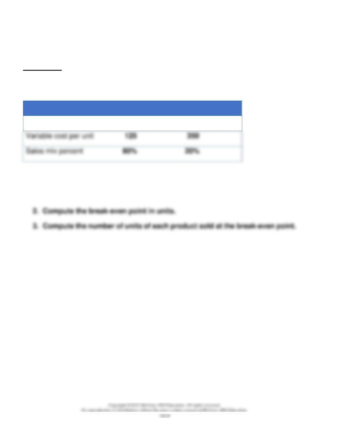
Handy Home sells window and doors and annual fixed costs of $900,000. Handy
Homes has the following information related to costs and sales mix:
Windows
Doors
Sales price per unit
$200
$500
125
350
Required:
1. Determine the weighted-average contribution margin per unit.
Financial and Managerial Accounting, 9th Edition
18–10
Chapter 18 Solution: Alternate Demo Problem #1
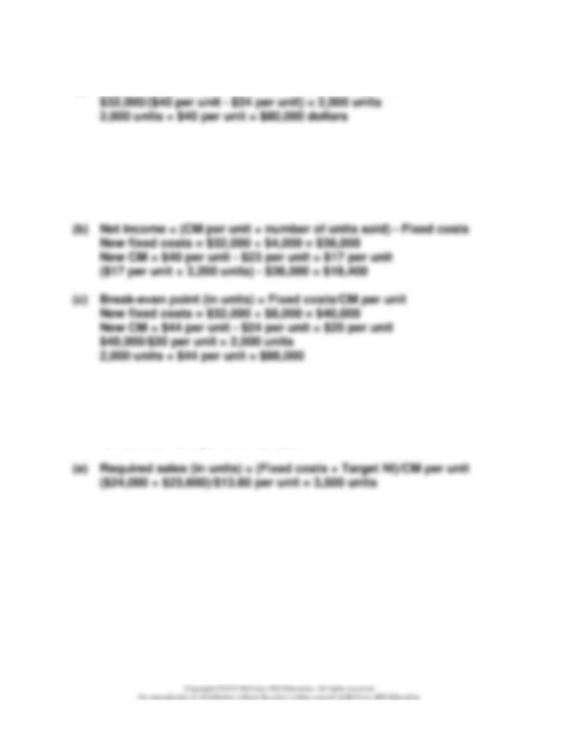
(a)
Break-even point (in units) = Fixed costs/CM per unit
$32,000/($40 per unit – $24 per unit) = 2,000 units
2,000 units × $40 per unit = $80,000 dollars
(or)
Break-even point (in dollars) = Fixed costs/CM ratio
$32,000/[($40 per unit –$16 per unit)/$40 per unit] = $80,000
$80,000 dollars/$40 per unit = 2,000 units
New fixed costs = $32,000 + $4,000 = $36,000
New CM = $40 per unit – $23 per unit = $17 per unit
($17 per unit × 3,200 units) – $36,000 = $18,400
(c)
Break-even point (in units) = Fixed costs/CM per unit
New fixed costs = $32,000 + $8,000 = $40,000
New CM = $44 per unit – $24 per unit = $20 per unit
$40,000/$20 per unit = 2,000 units
2,000 units × $44 per unit = $88,000
(d)
Break-even point (in units) = Fixed costs/CM per unit
New fixed costs = $32,000 – $8,000 = $24,000
New CM = $40 per unit – $26.40 per unit = $13.60 per unit
$24,000/$13.60 per unit = 1,765 units
1,765 units × $40 per unit = $70,600
(e)
Required sales (in units) = (Fixed costs + Target NI)/CM per unit
($24,000 + $23,600)/$13.60 per unit = 3,500 units
Financial and Managerial Accounting, 9th Edition
18–11
Chapter 18 Solution: Alternate Demo Problem #2
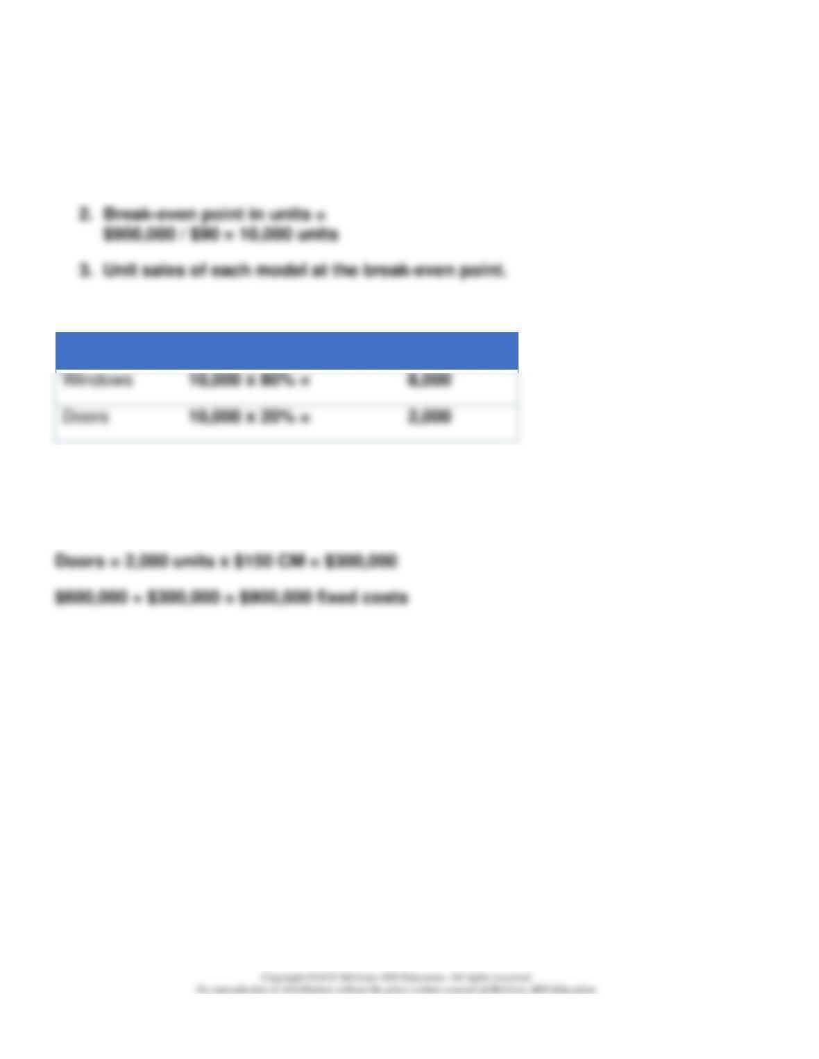
1. Weighted-average contribution margin per unit =
($75 x 80%) + ($150 x 20%) = $90
Model
Break-even Units x Mix
Units
Check:
Windows = 8,000 units x $75 CM = $600,000